Case Studies - not finished

Last updated: 2018-01-08

Code version: ca6e6f8

NB Not finished

Please note that this is hasty work, most of the assignments are not thoroughly answered.

Instructions

Use the morning to examine the datasets for the case studies. For each case: 1. get the appropriate descriptive statistics; 2. form an analysis plan; 3. try to develop a sense (“gut feeling”) of what the results of the analysis will be; and 4. if you have time, perform a full analysis on at least one case.

Remember the “Steps of Data Analysis” presented on the first day of the course!

You may work on your own or in a group, at your own computer or at the scheduled location, or in one of the computer rooms (if available) or in ‘Studielandschap’. Note that there is no assistance available during the morning.

During the lecture (13.30 to 17.00 at the very latest) we will discuss the analysis of the cases. There will also be plenty of time for you to ask questions.

The Case Studies

Case Study 1: fruitflies

For female fruitflies it is known that increased reproduction leads to a shortened life span. For male fruitflies this has never been ascertained. Male fruitflies that mate on average once a day are known to live for 60 days. The question is whether manipulation of sexual activity influences life span. To answer this question the following experiment was done: For one specific species of fruitflies, sexual activity was manipulated by providing individual males with either one or eight receptive, virginal females per day. Further, individual males were provided with one or eight recently inseminated females (these females do not wish to be inseminated again). A number of males were kept solitarily. Relevant variables were coded as follows: The data are given in the file fruitfly.sav or fruitfly.RData

variable	explanation
number	number of females provided
type	type of company (0: recently inseminated, 1: virginal, 9: none)
day	day=0 if life span is shorter than 60 days, day=1 if life span is longer than 60 days
thorax	thorax length of male
sleep	average percentage of time spent sleeping per day

Research objective

Answer the question: do male fruitflies have a shorte life span when they reproduce more?

Variables of interest

determinant: number AND type
outcome: day
possible confounders: thorax, sleep

Number and type will be included, as they will together determine how many times a male fruitfly may reproduce. Thorax and sleep are included, because both could be related to the outcome, and possibly the determinant.

Data exploration

load(epistats::fromParentDir("data/fruitfly.RData"))
str(fruitfly)

'data.frame':   125 obs. of  5 variables:
 $ NUMBER: num  0 0 0 0 0 0 0 0 0 0 ...
 $ TYPE  : Factor w/ 3 levels "recently inseminated",..: 3 3 3 3 3 3 3 3 3 3 ...
 $ DAY   : Factor w/ 2 levels "shorter than 60 days",..: 1 1 1 1 1 1 2 1 1 2 ...
 $ THORAX: num  0.64 0.7 0.72 0.72 0.72 0.76 0.78 0.8 0.84 0.84 ...
 $ SLEEP : num  18 6 19 7 16 13 35 2 35 6 ...

Data curation

Number is coded as numeric. However, it only has two distinct values: 0 and 8. It may be better to recode this as a categorical variable.

table(fruitfly$NUMBER)


 0  1  8 
25 50 50

# fruitfly$NUMBER <- factor(fruitfly$NUMBER)

Pairs plot

require(GGally)
GGally::ggpairs(fruitfly)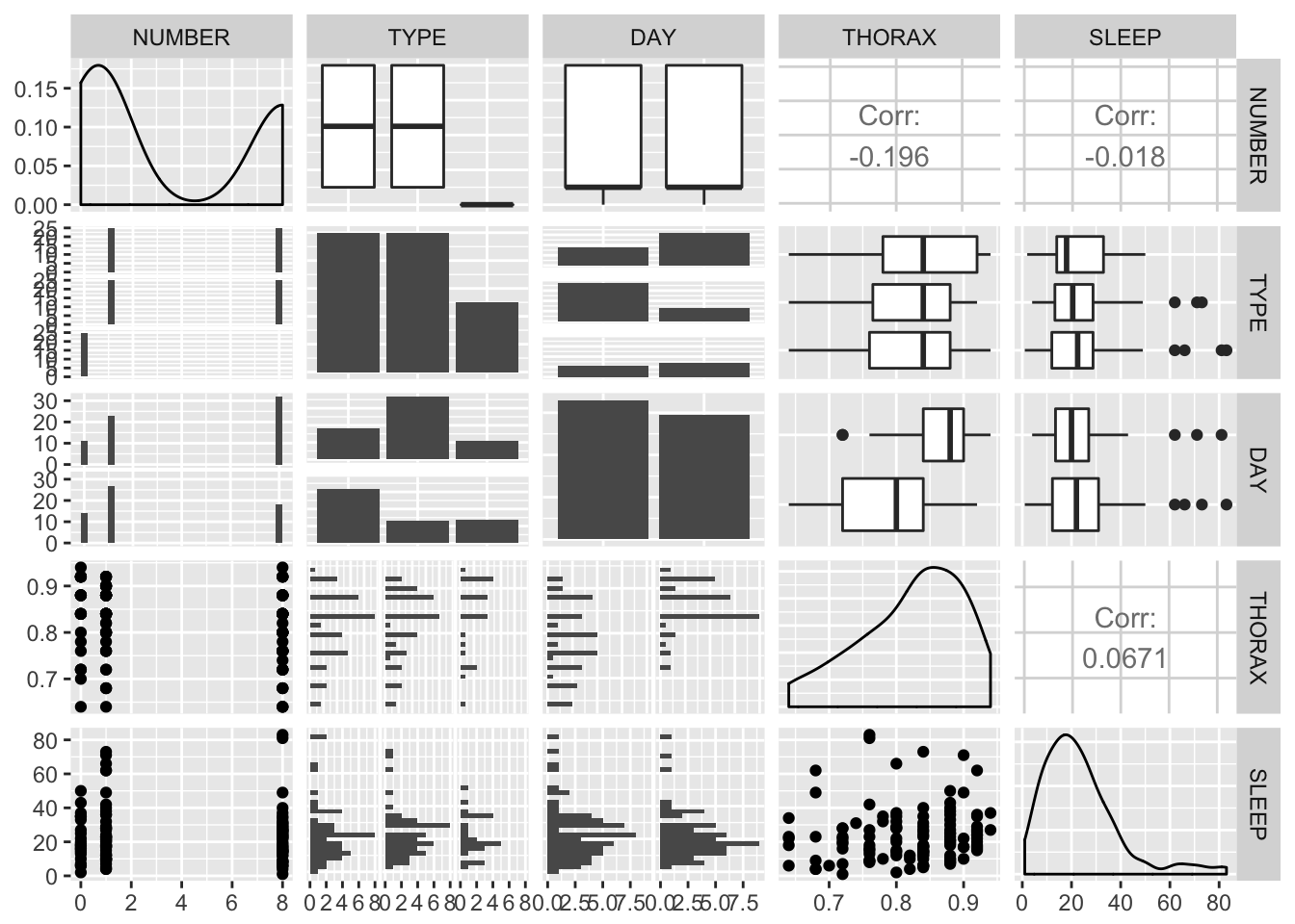

From this exploratory analysis we can observe Day seems to be associated with thorax, and maybe with number and type too.

The distribution of thorax is a little left-skewed, while sleep is somewhat right-skewed.

Analysis plan

Day is a binary outcome, we are interested in the rate of Day > 60. For univariate analysis, we can create a contingency table and perform a chi-squared test, for multivariate analysis we can use logistic regression. As this is an etiologic question, we will include all possible confounders in the multiple regression model. We expect that type may modify the effect of number (as this determines the number of available mates), so we will include an interaction term with type and number.

Other possibility: recode number and type into 5 groups, do chi-squared

Interpretation of results

Crude analysis

tab <- xtabs(~NUMBER+DAY, data = fruitfly)
tab

      DAY
NUMBER shorter than 60 days longer than 60 days
     0                   11                  14
     1                   23                  27
     8                   32                  18

prop.table(tab, margin = 1)

      DAY
NUMBER shorter than 60 days longer than 60 days
     0                 0.44                0.56
     1                 0.46                0.54
     8                 0.64                0.36

chisq.test(tab)


    Pearson's Chi-squared test

data:  tab
X-squared = 4.2212, df = 2, p-value = 0.1212

In crude analysis, there seems to be no statistically significant association between day and number.

Multiple regression

fit <- glm(DAY~NUMBER*TYPE+THORAX+SLEEP, data = fruitfly, family = binomial)
fit_scaled <- glm(DAY~NUMBER*TYPE+scale(THORAX, center = T, scale = T)+SLEEP, data = fruitfly, family = binomial)
fit_parsimonious <- glm(DAY~NUMBER*TYPE, data = fruitfly, family = binomial)
summary(fit)


Call:
glm(formula = DAY ~ NUMBER * TYPE + THORAX + SLEEP, family = binomial, 
    data = fruitfly)

Deviance Residuals: 
     Min        1Q    Median        3Q       Max  
-2.05883  -0.49334  -0.06449   0.67281   2.08158  

Coefficients: (1 not defined because of singularities)
                     Estimate Std. Error z value Pr(>|z|)    
(Intercept)         -18.04235    3.97107  -4.543 5.53e-06 ***
NUMBER                0.18537    0.11444   1.620  0.10527    
TYPEvirginal         -0.31544    0.81062  -0.389  0.69718    
TYPEnone             -0.33237    0.77118  -0.431  0.66648    
THORAX               22.82644    4.73746   4.818 1.45e-06 ***
SLEEP                -0.02389    0.01449  -1.649  0.09917 .  
NUMBER:TYPEvirginal  -0.63327    0.20464  -3.095  0.00197 ** 
NUMBER:TYPEnone            NA         NA      NA       NA    
---
Signif. codes:  0 '***' 0.001 '**' 0.01 '*' 0.05 '.' 0.1 ' ' 1

(Dispersion parameter for binomial family taken to be 1)

    Null deviance: 172.89  on 124  degrees of freedom
Residual deviance: 100.82  on 118  degrees of freedom
AIC: 114.82

Number of Fisher Scoring iterations: 6

summary(fit_parsimonious)


Call:
glm(formula = DAY ~ NUMBER * TYPE, family = binomial, data = fruitfly)

Deviance Residuals: 
    Min       1Q   Median       3Q      Max  
-1.5096  -1.1436  -0.2857   1.0108   2.5373  

Coefficients: (1 not defined because of singularities)
                     Estimate Std. Error z value Pr(>|z|)   
(Intercept)          0.355707   0.470573   0.756  0.44971   
NUMBER               0.049758   0.084575   0.588  0.55631   
TYPEvirginal         0.006823   0.672310   0.010  0.99190   
TYPEnone            -0.114545   0.619497  -0.185  0.85331   
NUMBER:TYPEvirginal -0.492331   0.177963  -2.766  0.00567 **
NUMBER:TYPEnone            NA         NA      NA       NA   
---
Signif. codes:  0 '***' 0.001 '**' 0.01 '*' 0.05 '.' 0.1 ' ' 1

(Dispersion parameter for binomial family taken to be 1)

    Null deviance: 172.89  on 124  degrees of freedom
Residual deviance: 142.31  on 120  degrees of freedom
AIC: 152.31

Number of Fisher Scoring iterations: 5

lmtest::lrtest(fit)

Likelihood ratio test

Model 1: DAY ~ NUMBER * TYPE + THORAX + SLEEP
Model 2: DAY ~ 1
  #Df  LogLik Df  Chisq Pr(>Chisq)    
1   7 -50.411                         
2   1 -86.447 -6 72.073  1.535e-13 ***
---
Signif. codes:  0 '***' 0.001 '**' 0.01 '*' 0.05 '.' 0.1 ' ' 1

drop1(fit)

Single term deletions

Model:
DAY ~ NUMBER * TYPE + THORAX + SLEEP
            Df Deviance    AIC
<none>           100.82 114.82
THORAX       1   141.07 153.07
SLEEP        1   103.75 115.75
NUMBER:TYPE  1   113.88 125.88

Longevity can partly be explained by the provided model. The length of the male (THORAX) seems to by the most important factor, fruitflies that are longer seem to live longer.
Number on itself is not significantly associated with the outcome. However from the interaction term, we see that the number of virginal female fruitflies is associated with shorter survival. Sleep does not seem to contribute significantly to the model.

Conclusions

Male fruitlies that reproduce more often seem to have a shorter life-span. However, the size of the thorax of the fruitfly is a more important predictor, with larger fruitflies living longer.

Case Study 2, Heroin rehab clinic

Caplehorn (1991) was interested in factors that have an effect on the success probability of retention of heroin addicts in a clinic. In a multi-center study he collected the following data from 238 heroin addicts. The data are given in the file heroin.sav or heroin.RData.

variable	explanation
ID	Identification code
CLINIC	Number of clinic (1 or 2)
STATUS	Status (0=not (yet) departed; 1= departed from clinic)
TIMES	Time in days that heroin addicts spent in the clinic
PRISON	Prison record (1=yes; 0=no)
DOSE	Methadone dosage in mg/day

(Source: Caplehorn J., 1991, Methadone dosage and retention of patients in maintenance treatment, Medical Journal of Australia, 154, 195 99)

The researchers are only interested in the effect of each explanatory variable separately. Would you advise further statistical analysis?

Research objective

Research question

What factors are associated with retention of heroin addicts in a clinic.

Variables of interest

determinants: CLINIC, TIMES, PRISON, DOSE
outcome: STATUS
possible confounders:

Data exploration

load(epistats::fromParentDir("data/heroin.RData"))
str(heroin)

'data.frame':   238 obs. of  6 variables:
 $ ID    : num  1 2 3 4 5 6 7 8 9 10 ...
 $ CLINIC: num  1 1 1 1 1 1 1 1 1 1 ...
 $ STATUS: num  1 1 1 1 1 1 1 0 1 1 ...
 $ TIMES : num  428 275 262 183 259 714 438 796 892 393 ...
 $ PRISON: num  0 1 0 0 1 0 1 1 0 1 ...
 $ DOSE  : num  50 55 55 30 65 55 65 60 50 65 ...

Data curation

Let’s throw out ID, since it is uninformative and throwing it out means that we don’t have to do that each time in the analysis

Clinic, status and prison should be coded as factor variables

heroin$ID <- NULL

require(dplyr)
heroin <- heroin %>%
  mutate_at(.vars = c("CLINIC", "STATUS", "PRISON"), factor)

str(heroin)

'data.frame':   238 obs. of  5 variables:
 $ CLINIC: Factor w/ 2 levels "1","2": 1 1 1 1 1 1 1 1 1 1 ...
 $ STATUS: Factor w/ 2 levels "0","1": 2 2 2 2 2 2 2 1 2 2 ...
 $ TIMES : num  428 275 262 183 259 714 438 796 892 393 ...
 $ PRISON: Factor w/ 2 levels "0","1": 1 2 1 1 2 1 2 2 1 2 ...
 $ DOSE  : num  50 55 55 30 65 55 65 60 50 65 ...

Pairs plot

require(ggplot2)
GGally::ggpairs(heroin)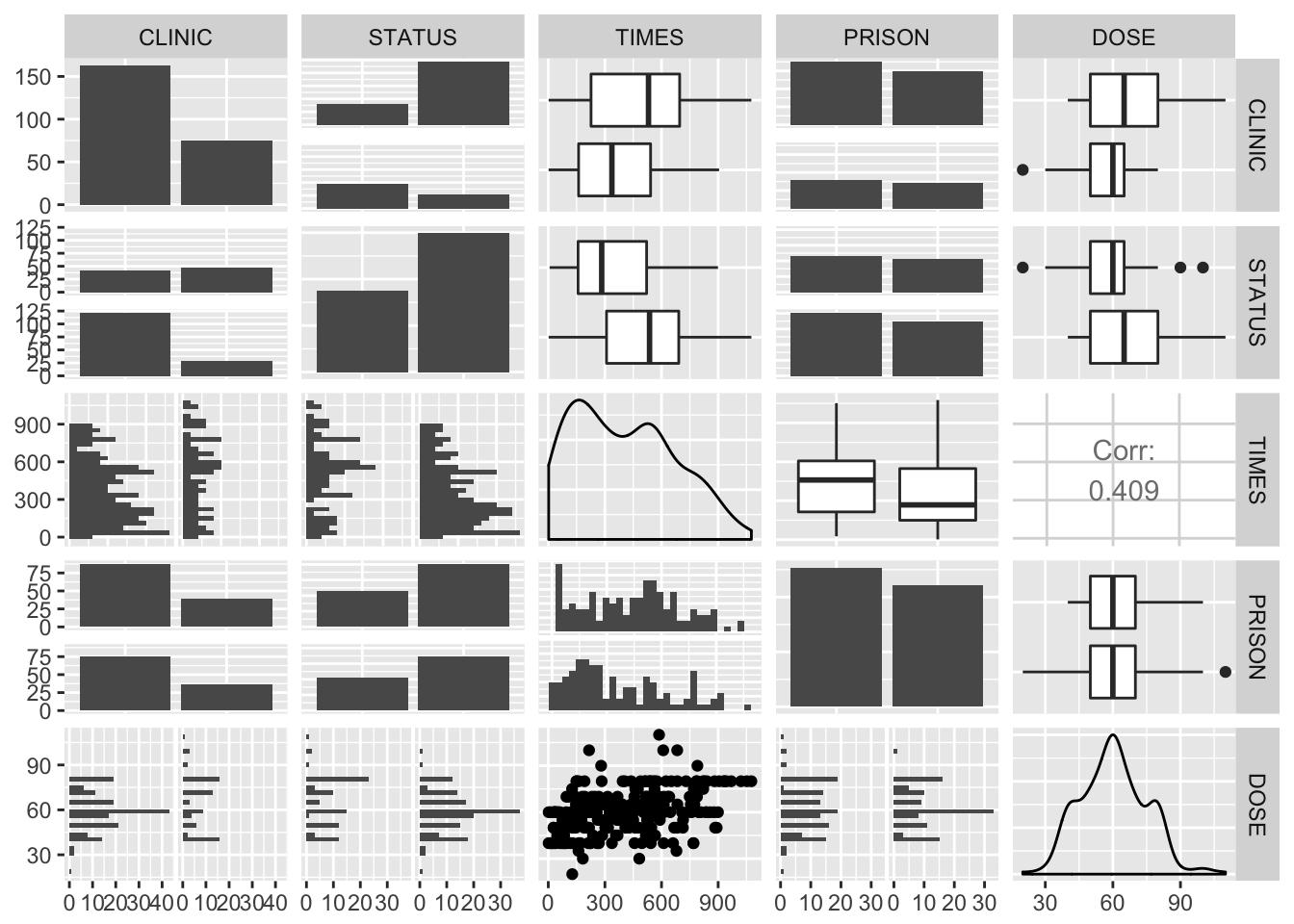

Satus seems to be related with times, clinic, and maybe prison. However, clinic and times also seem to be related, so it could be that one of them explains the effect of the other. Also, TIMES and DOSE seem to be associated with each other.

Analysis plan

We will use multiple logistic-regression analysis, as the effect of any single factor (or lack thereof) may be confounded by other factors.

Better plan: treat as survival data, predict how long they stay

require(survival)
surv_obj <- Surv(time = heroin$TIMES, event = heroin$STATUS)
km_fit <- survfit(Surv(time = TIMES, event = STATUS==1)~1, data = heroin)
plot(km_fit)

lines(survfit(Surv(time = TIMES, event = STATUS==1)~CLINIC, data = heroin),
     main = "retention by clinic", col = c("red", "blue"))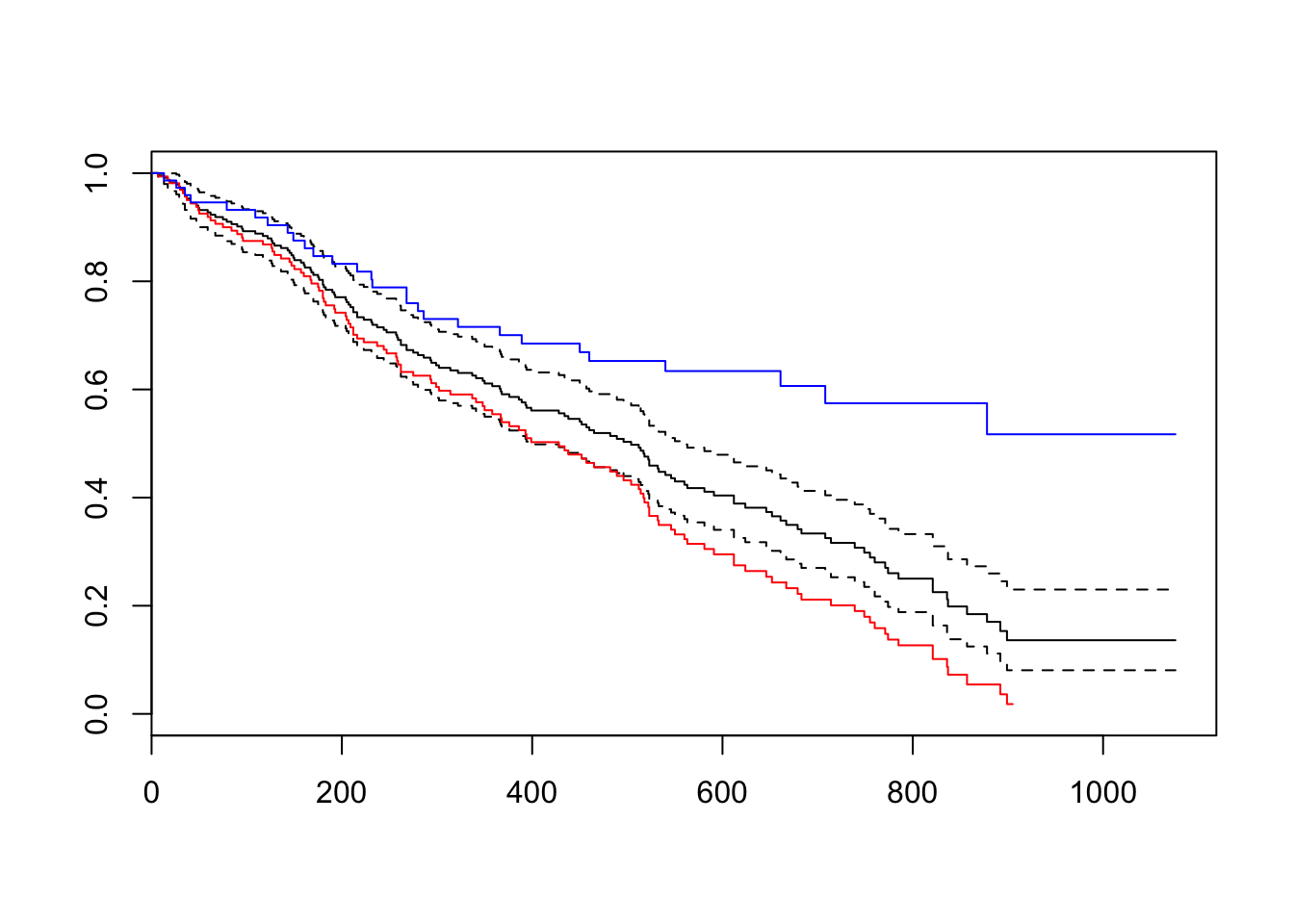

plot(survfit(Surv(time = TIMES, event = STATUS==1)~CLINIC, data = heroin),
     main = "retention by prison", col = c("red", "blue"))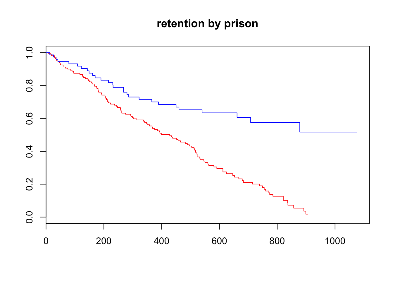

plot(survfit(Surv(time = TIMES, event = STATUS==1)~epistats::quant(DOSE), data = heroin),
     main = "retention by quantiles of dose", lty = 1:4)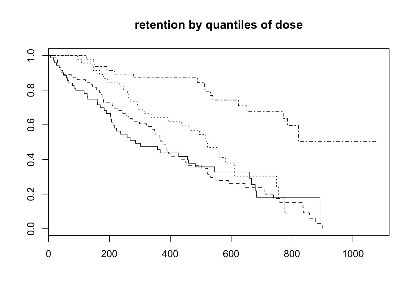

cox_fit <- coxph(Surv(time = TIMES, event = STATUS==1)~CLINIC+PRISON+DOSE, data = heroin)
summary(cox_fit)

Call:
coxph(formula = Surv(time = TIMES, event = STATUS == 1) ~ CLINIC + 
    PRISON + DOSE, data = heroin)

  n= 238, number of events= 150 

             coef exp(coef)  se(coef)      z Pr(>|z|)    
CLINIC2 -1.009896  0.364257  0.214889 -4.700 2.61e-06 ***
PRISON1  0.326555  1.386184  0.167225  1.953   0.0508 .  
DOSE    -0.035369  0.965249  0.006379 -5.545 2.94e-08 ***
---
Signif. codes:  0 '***' 0.001 '**' 0.01 '*' 0.05 '.' 0.1 ' ' 1

        exp(coef) exp(-coef) lower .95 upper .95
CLINIC2    0.3643     2.7453    0.2391    0.5550
PRISON1    1.3862     0.7214    0.9988    1.9238
DOSE       0.9652     1.0360    0.9533    0.9774

Concordance= 0.665  (se = 0.026 )
Rsquare= 0.238   (max possible= 0.997 )
Likelihood ratio test= 64.56  on 3 df,   p=6.228e-14
Wald test            = 54.12  on 3 df,   p=1.056e-11
Score (logrank) test = 56.32  on 3 df,   p=3.598e-12

We can use logrank test for 2 groups

Crude analysis

Multiple regression

Interpretation of results

Conclusions

Case Study 3, Maternal mortality rates

Researchers examined maternal mortality rates (MMRs) in relation to the global distribution of physicians and nurses. A UN database on 155 countries was constructed in order to determine whether MMRs were related to the proportion of births attended by medical and nonmedical staff (defined as “attendance at birth by trained personnel” (physicians, nurses, midwives or primary health care workers trained in midwifery skills), the ratio of physicians and nurses to the population, female literacy and gross national product (GNP) per capita. The data are given in the file maternalmort.sav or maternalmort.RData.

variable	explanation
Country	name of country
Physician	physicians per 1000 population
Nurses	nurses per 1000 population
GNP	gross national product per capita in dollars
MMR	maternal mortality rate (per 100,000 births)
Attended	births attended by trained personnel (%)
Femlit	female literacy (%)

Research objective

Research question

What is the relationship between the proportion of births attended by trained medical staff and maternal mortality rates, adjusted for gross national product per capita and female literacy

Variables of interest

determinant: Attended
outcome: MMR
possible confounders: Physician, Nurses, GNP, Femlit

Data exploration

load(epistats::fromParentDir("data/maternalmort.RData"))
str(maternalmort)

'data.frame':   152 obs. of  7 variables:
 $ Country  : Factor w/ 152 levels "Afghanistan",..: 1 2 3 4 5 6 7 8 9 10 ...
 $ physician: num  0.1 1.4 0.8 0.07 0.9 2.7 3.1 2.2 2.6 3.9 ...
 $ nurses   : num  0.1 4.7 3.2 16.4 4.8 2.1 6.4 8.5 8.4 10.8 ...
 $ GNP      : num  280 670 1600 700 6770 ...
 $ MMR      : num  1700 65 160 1500 NA 100 50 9 10 22 ...
 $ attended : num  9 99 77 15 NA 97 NA 100 100 NA ...
 $ femlit   : num  15 NA 49 29 NA 96 98 NA NA 96 ...

Data curation

Pairs plot

GGally::ggpairs(maternalmort[, -1])

Warning: Removed 6 rows containing non-finite values (stat_density).

Warning in (function (data, mapping, alignPercent = 0.6, method =
"pearson", : Removed 9 rows containing missing values

Warning in (function (data, mapping, alignPercent = 0.6, method =
"pearson", : Removed 6 rows containing missing values

Warning in (function (data, mapping, alignPercent = 0.6, method =
"pearson", : Removed 15 rows containing missing values

Warning in (function (data, mapping, alignPercent = 0.6, method =
"pearson", : Removed 41 rows containing missing values

Warning in (function (data, mapping, alignPercent = 0.6, method =
"pearson", : Removed 44 rows containing missing values

Warning: Removed 9 rows containing missing values (geom_point).

Warning: Removed 6 rows containing non-finite values (stat_density).

Warning in (function (data, mapping, alignPercent = 0.6, method =
"pearson", : Removed 6 rows containing missing values

Warning in (function (data, mapping, alignPercent = 0.6, method =
"pearson", : Removed 15 rows containing missing values

Warning in (function (data, mapping, alignPercent = 0.6, method =
"pearson", : Removed 41 rows containing missing values

Warning in (function (data, mapping, alignPercent = 0.6, method =
"pearson", : Removed 44 rows containing missing values

Warning: Removed 6 rows containing missing values (geom_point).

Warning: Removed 6 rows containing missing values (geom_point).

Warning in (function (data, mapping, alignPercent = 0.6, method =
"pearson", : Removed 9 rows containing missing values

Warning in (function (data, mapping, alignPercent = 0.6, method =
"pearson", : Removed 35 rows containing missing values

Warning in (function (data, mapping, alignPercent = 0.6, method =
"pearson", : Removed 38 rows containing missing values

Warning: Removed 15 rows containing missing values (geom_point).

Warning: Removed 15 rows containing missing values (geom_point).

Warning: Removed 9 rows containing missing values (geom_point).

Warning: Removed 9 rows containing non-finite values (stat_density).

Warning in (function (data, mapping, alignPercent = 0.6, method =
"pearson", : Removed 35 rows containing missing values

Warning in (function (data, mapping, alignPercent = 0.6, method =
"pearson", : Removed 38 rows containing missing values

Warning: Removed 41 rows containing missing values (geom_point).

Warning: Removed 41 rows containing missing values (geom_point).

Warning: Removed 35 rows containing missing values (geom_point).

Warning: Removed 35 rows containing missing values (geom_point).

Warning: Removed 35 rows containing non-finite values (stat_density).

Warning in (function (data, mapping, alignPercent = 0.6, method =
"pearson", : Removed 52 rows containing missing values

Warning: Removed 44 rows containing missing values (geom_point).

Warning: Removed 44 rows containing missing values (geom_point).

Warning: Removed 38 rows containing missing values (geom_point).

Warning: Removed 38 rows containing missing values (geom_point).

Warning: Removed 52 rows containing missing values (geom_point).

Warning: Removed 38 rows containing non-finite values (stat_density).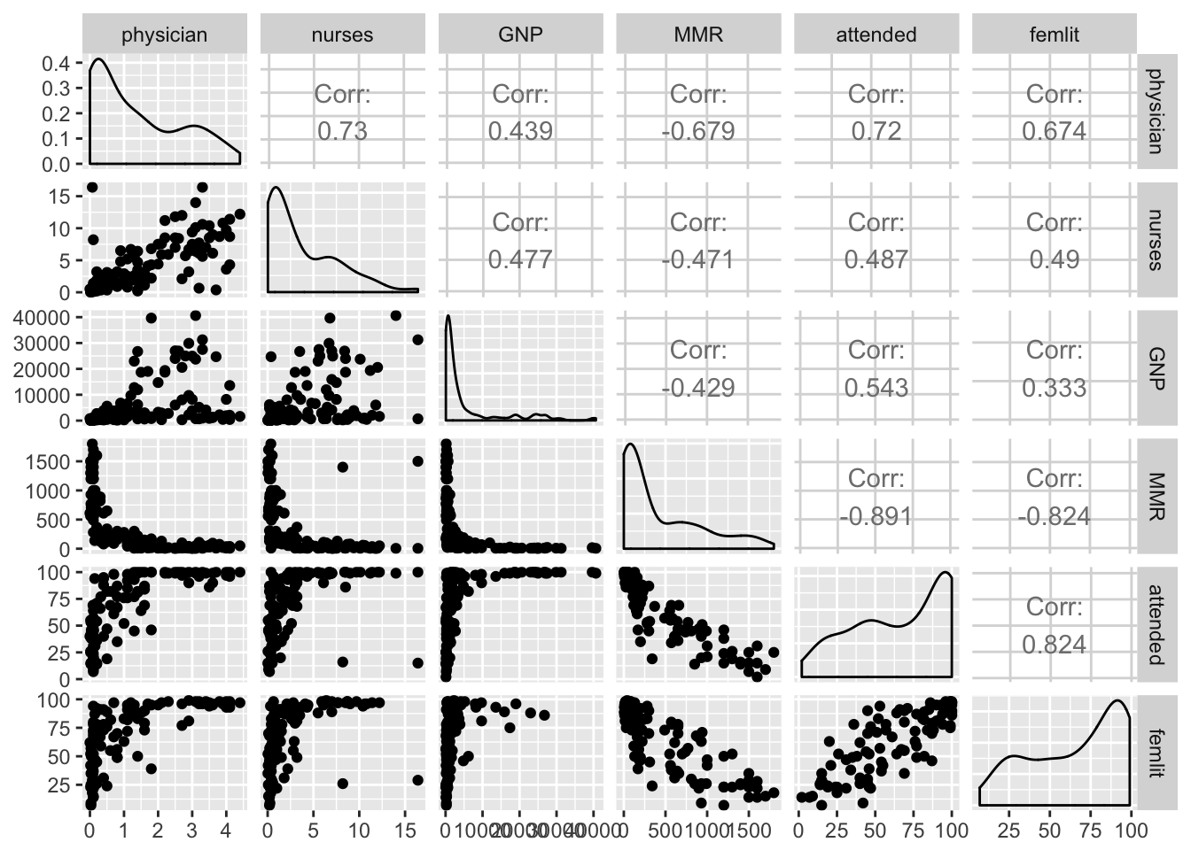

require(dplyr)
maternalmort %>%
  mutate_at(.vars = c("physician", "nurses", "GNP"), function(x) log(x+.01)) %>%
  select(-Country) %>%
  GGally::ggpairs()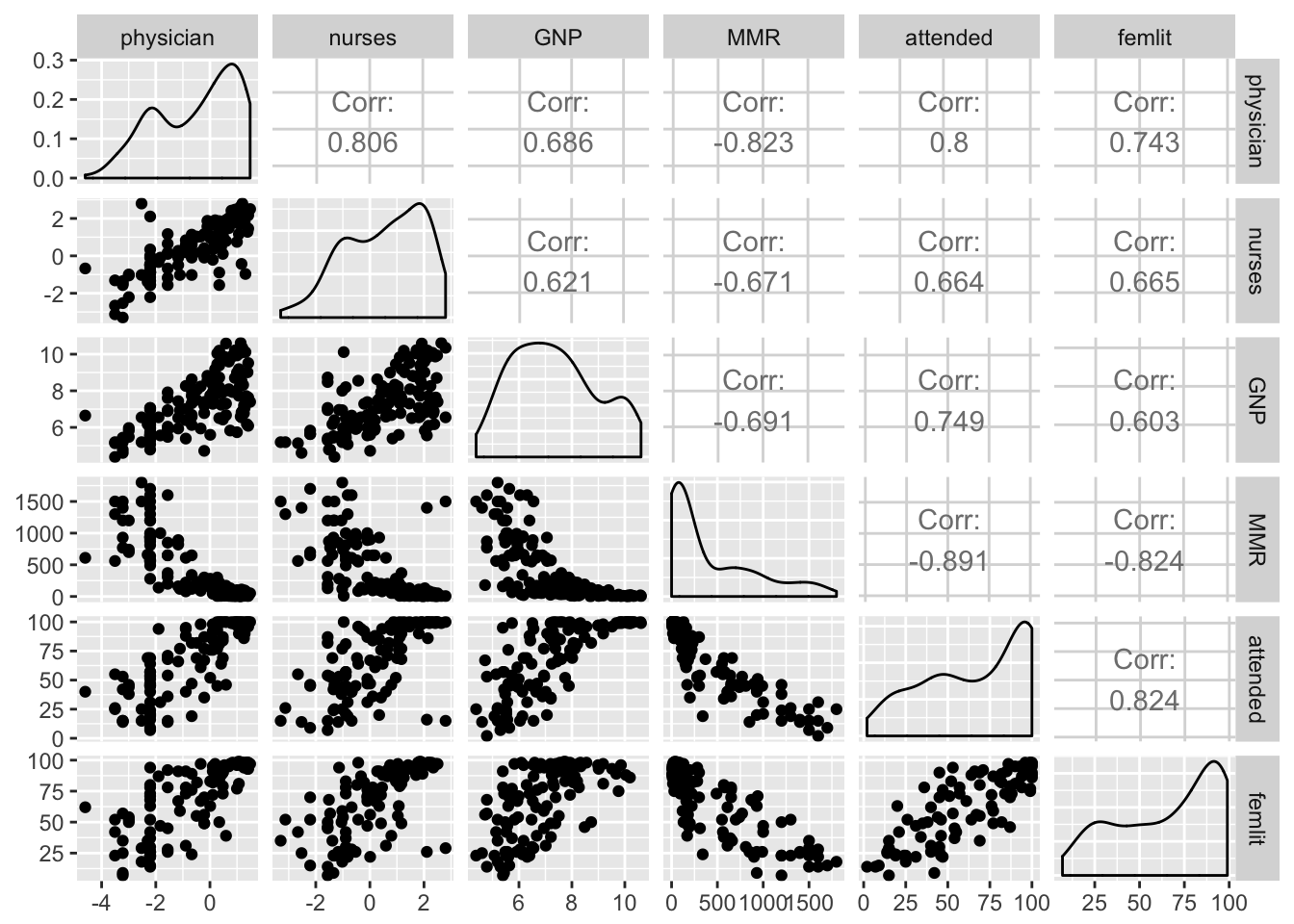

Looks like strong collinearity for attended and femlit

Analysis plan

We are trying to model a continous variable: MMR. Strictly speaking it is a rate, which should optimally be modeled with Poisson regression, however we do not have the original counts. However for large enough rates, the poisson distribution opproximates the normal distribution, so we can also use (multiple) linear regression.

Crude analysis

Multiple regression

fit1 <- maternalmort %>%
  mutate_at(.vars = c("physician", "nurses", "GNP"), 
            function(x) log(x + 0.01)) %>%
  select(-Country) %>%
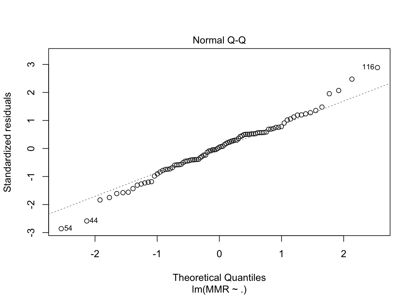
  lm(MMR~., data = .)

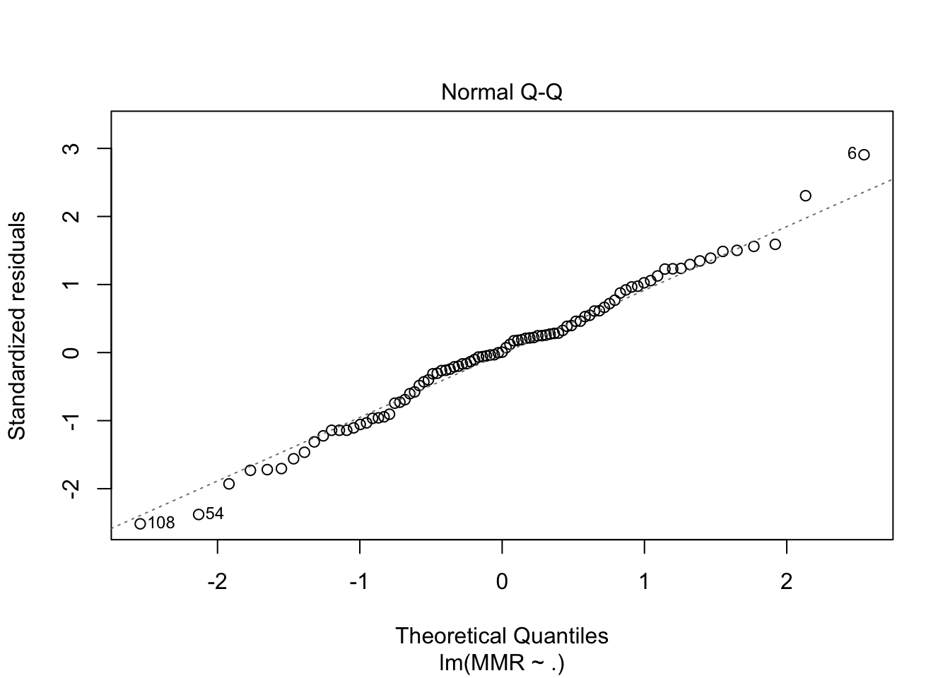
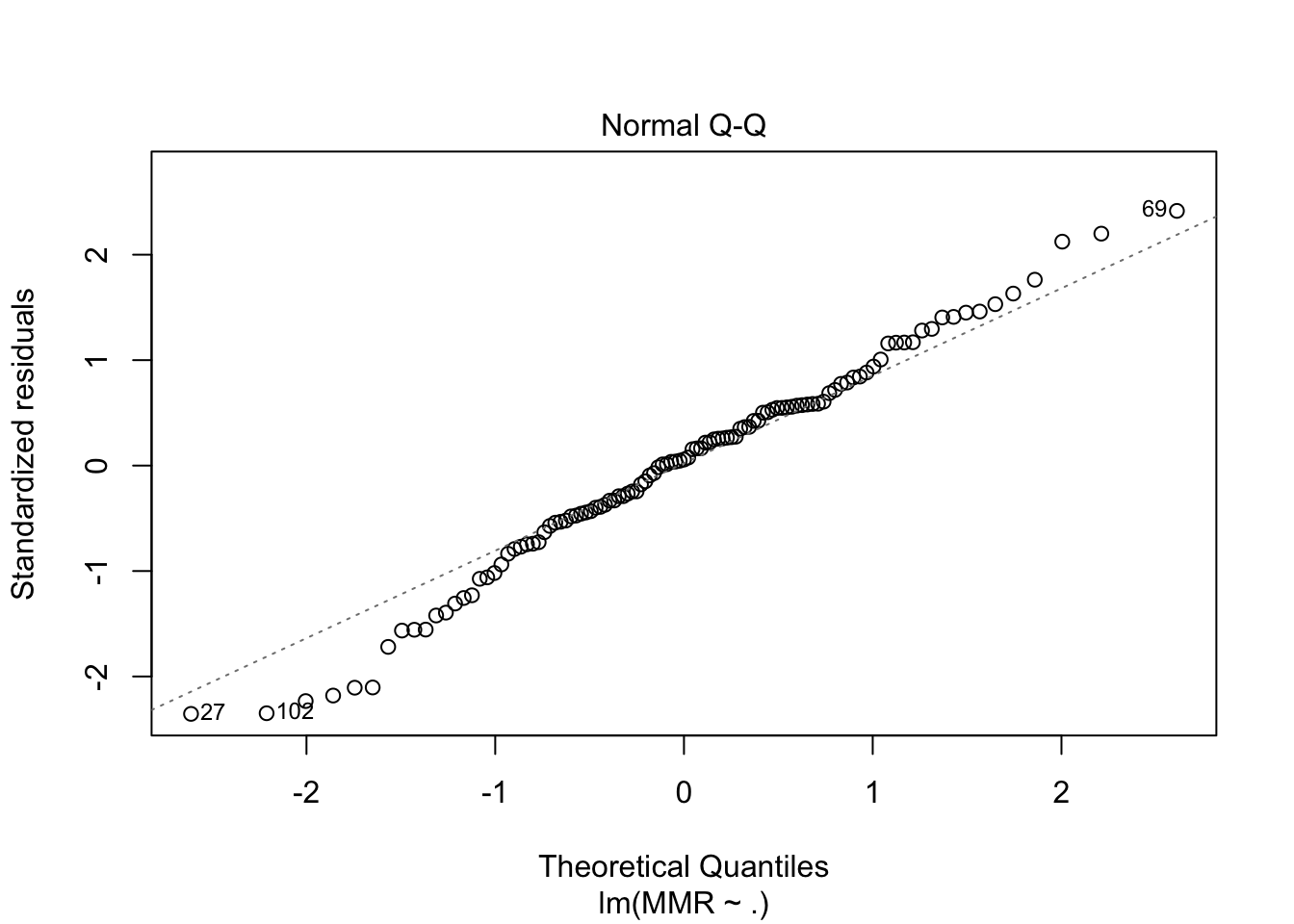
plot(fit1, which = c(1,2))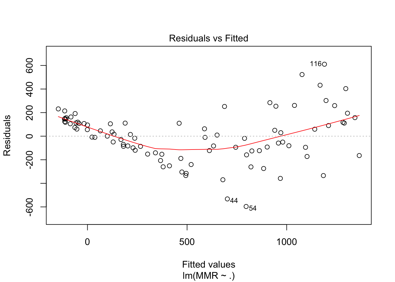

fit2 <- maternalmort %>%
  mutate_at(.vars = c("physician", "nurses", "GNP", "MMR"), 
            function(x) log(x + 0.01)) %>%
  select(-Country) %>%
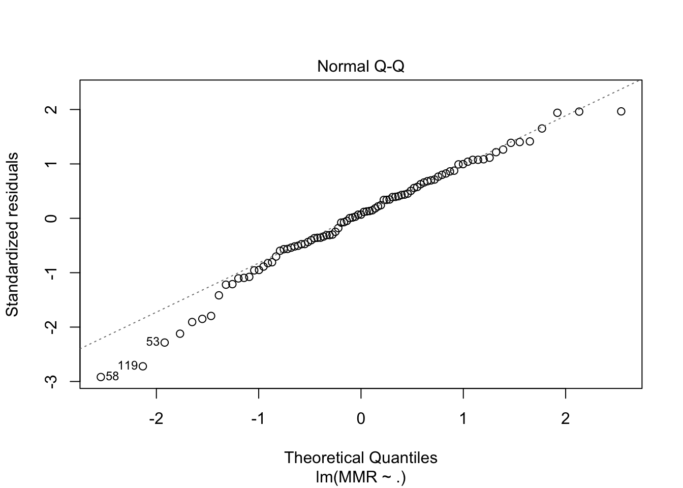
  lm(MMR~., data = .)

plot(fit2, which = c(1,2))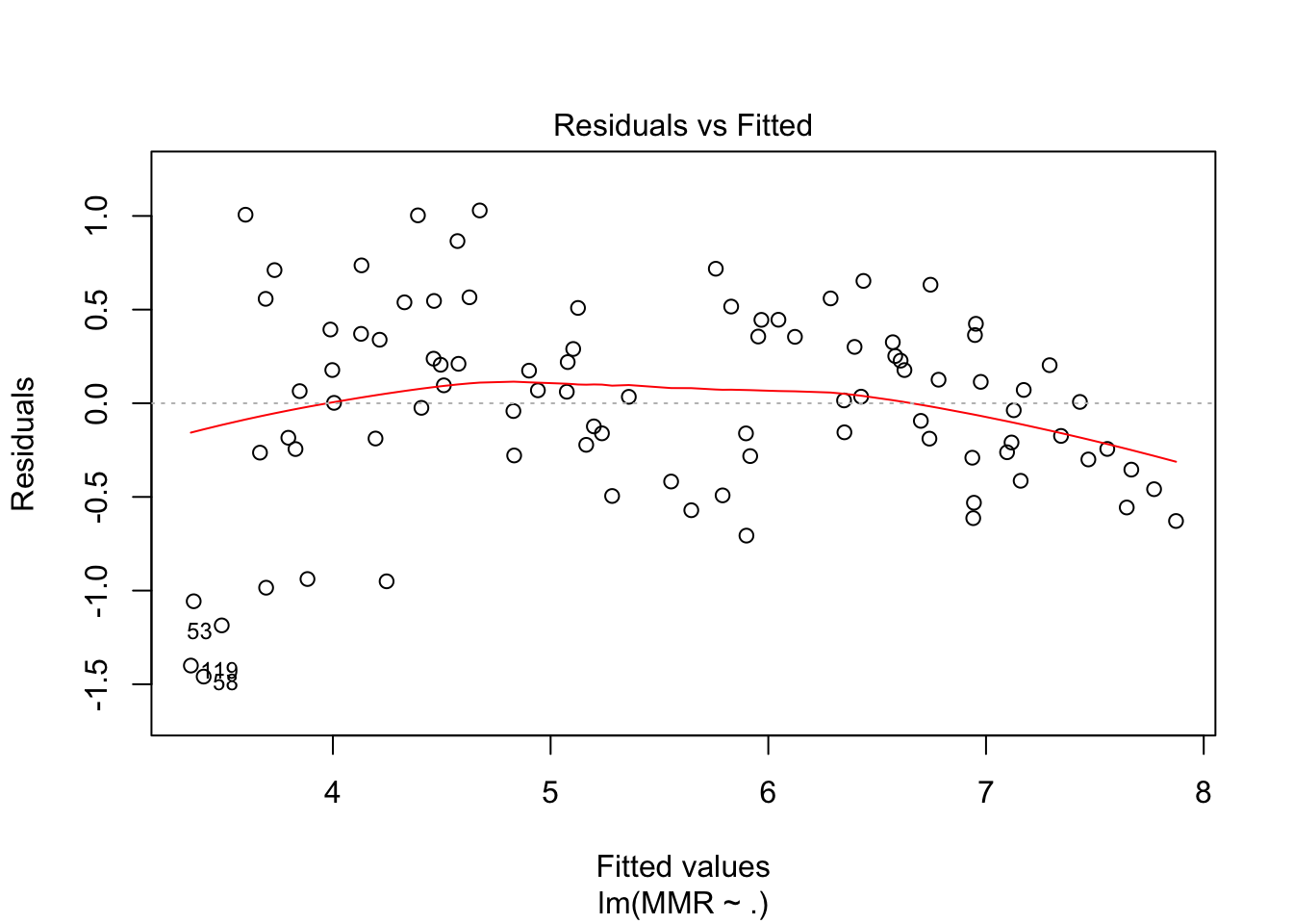

fit3 <- maternalmort %>%
  mutate_at(.vars = c("MMR"), 
            function(x) log(x + 0.01)) %>%
  select(-Country) %>%
  lm(MMR~., data = .)

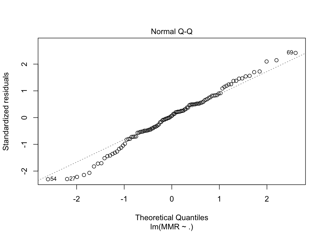
plot(fit3, which = c(1,2))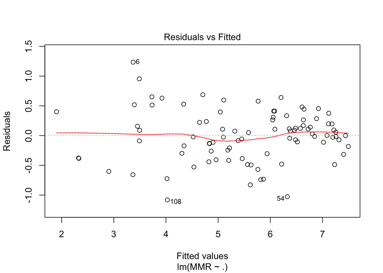

fit4 <- maternalmort %>%
  mutate_at(.vars = c("MMR"), 
            function(x) log(x + 0.01)) %>%
  select(-c(Country, femlit)) %>%
  lm(MMR~., data = .)

plot(fit4, which = c(1,2))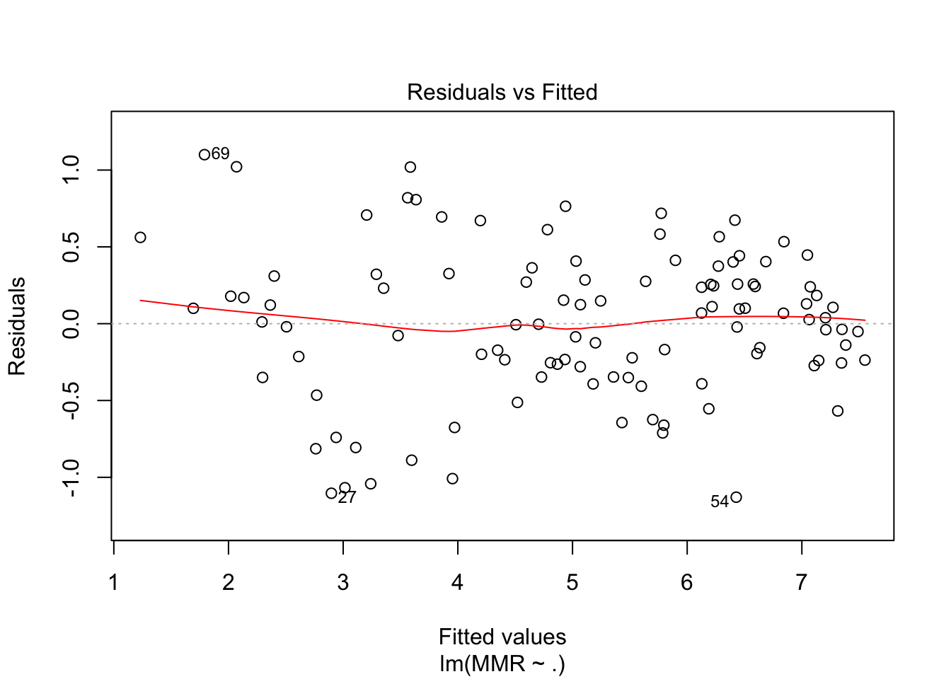

drop1(fit4, test = "F")

Single term deletions

Model:
MMR ~ physician + nurses + GNP + attended
          Df Sum of Sq    RSS      AIC  F value    Pr(>F)    
<none>                 25.385 -146.381                       
physician  1     7.150 32.535 -121.580  29.0115 4.565e-07 ***
nurses     1     0.085 25.470 -148.022   0.3431    0.5593    
GNP        1    21.927 47.312  -81.140  88.9686 1.354e-15 ***
attended   1    34.486 59.871  -55.714 139.9265 < 2.2e-16 ***
---
Signif. codes:  0 '***' 0.001 '**' 0.01 '*' 0.05 '.' 0.1 ' ' 1

fit5 <- maternalmort %>%
  mutate_at(.vars = c("MMR"), 
            function(x) log(x + 0.01)) %>%
  select(-c(Country, femlit, nurses)) %>%
  lm(MMR~., data = .)

plot(fit5, which = c(1,2))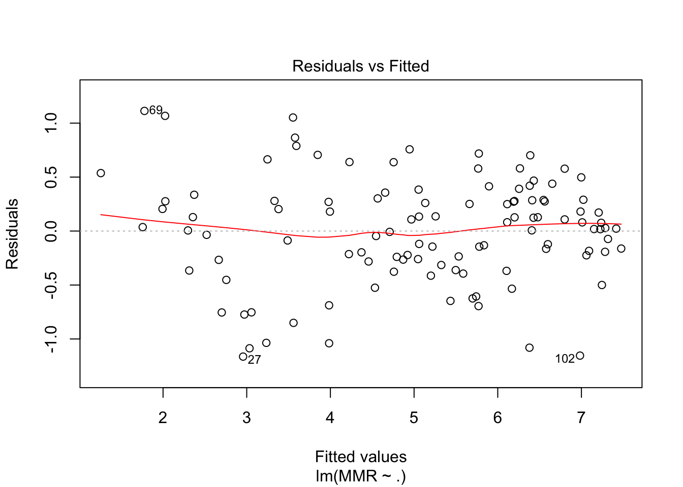

drop1(fit5, test = "F")

Single term deletions

Model:
MMR ~ physician + GNP + attended
          Df Sum of Sq    RSS      AIC F value    Pr(>F)    
<none>                 26.920 -149.250                      
physician  1    10.945 37.864 -113.382  43.502 1.659e-09 ***
GNP        1    26.908 53.828  -74.335 106.952 < 2.2e-16 ***
attended   1    33.281 60.201  -61.915 132.283 < 2.2e-16 ***
---
Signif. codes:  0 '***' 0.001 '**' 0.01 '*' 0.05 '.' 0.1 ' ' 1

1/car::vif(fit5)

physician       GNP  attended 
0.4447664 0.6613548 0.4530873

Interpretation of results

Look at Countries with highest residual, which means high rates, that is unexplained by the model.

resids <- fit5$residuals
ordered_resids <- sort(resids, decreasing = T)
included_observations <- names(ordered_resids)


data.frame(residual = ordered_resids,
           maternalmort[names(ordered_resids),])

        residual     Country physician nurses   GNP  MMR attended femlit
69   1.113069146 Japan            1.80  6.800 39640   18      100     NA
51   1.067351374 Germany          3.30  5.600 27510   22       99     NA
6    1.052036593 Argentina        2.70  2.100  8030  100       97     96
144  0.865275704 Uruguay          3.20  0.640  5170   85       96     98
71   0.789012445 Kazakhstan       3.60  9.000  1330   80       99     96
45   0.757207462 El Salvador      0.80  0.900  1610  300       87     70
126  0.718296284 Sudan            0.09  0.240   480  660       69     35
38   0.705648224 Cuba             3.60  6.100  1170   95       90     95
115  0.701652352 Senegal          0.10  0.260   600 1200       46     23
142  0.664098080 Ukraine          4.40 12.200  1630   50      100     97
110  0.639604948 Rumania          1.80  4.300  1480  130      100     95
21   0.638028247 Brazil           1.40  0.400  3640  220       81     83
151  0.580683795 Zambia           0.10  0.900   400  940       51     71
152  0.579279369 Zimbabwe         0.10  0.610   540  570       69     80
55   0.577919337 Guinea           0.10  0.430   550 1600       31     22
130  0.537043612 Switzerland      3.10 14.000 40630    6       99     NA
116  0.497468745 Sierra Leon      0.07  0.350   180 1800       25     18
17   0.467301051 Benin            0.10  0.580   370  990       45     26
141  0.438439274 Uganda           0.04  0.340   240 1200       38     50
25   0.419998176 Cambodia         0.10  1.000   270  900       47     22
26   0.414557174 Cameroon         0.10  0.640   650  550       64     52
134  0.391523647 Tanzania         0.03  0.220   120  770       53     57
113  0.384065205 South Afric      0.61  2.750  3160  230       82     82
70   0.356211483 Jordan           1.60  3.000  1510  150       87     79
49   0.336182249 France           2.80  5.700 24990   15       99     NA
114  0.302266526 Saudi Arabi      1.40  0.200  6180  130       82     50
92   0.290068913 Mozambique       0.02  0.260    80 1500       25     23
23   0.288029677 Burkina          0.03  0.250   230  930       42      9
36   0.285252701 Cote d'Ivoi      0.10  0.400   660  810       45     30
14   0.279362455 Belarus          4.10 11.400  2070   37      100     97
19   0.277879185 Bolivia          0.50  0.900   800  650       47     76
15   0.276141597 Belgium          3.70  0.370 24710   10      100     NA
87   0.274492451 Mauritania       0.10  0.500   460  930       40     26
136  0.272138959 Togo             0.10  0.400   310  640       54     37
73   0.270084243 Korean Rep.      1.20  6.700  9700   70       98     97
57   0.260159551 Honduras         0.40  1.200   600  220       88     73
94   0.251001887 Namibia          0.20  3.200  2000  370       68     NA
93   0.249562379 Mynamar          0.10  0.400   220  580       57     78
40   0.204947002 Denmark          2.90  6.700 29890    9      100     NA
81   0.203738431 Lithuania        4.00  9.700  1900   36      100     98
112  0.180603328 Rwanda           0.02  0.034   180 1300       26     52
90   0.180054616 Mongolia         2.70     NA   310   65       99     77
18   0.171473569 Bhutan           0.20  0.500   420 1600       15     28
80   0.136248786 Libya            1.00  2.900   269  220       76     63
139  0.134129903 Turkey           1.10  1.500  2780  180       76     72
145  0.129025681 USA              2.50  7.000 26980   12       99     NA
52   0.127929948 Ghana            0.04  0.360   390  740       44     54
84   0.126980434 Malawi           0.02  0.060   170  560       55     42
28   0.123577525 Central Afr      0.04  0.100   340  700       46     52
99   0.107958020 Nigeria          0.15  0.900   260 1000       31     47
148  0.107754470 Vietnam          0.40  2.300   219  160       95     91
82   0.081584905 Madagasca        0.10  0.400   230  490       57     73
85   0.080482609 Mali             0.10  0.250   250 1200       24     23
4    0.076400972 Angola           0.07 16.400   700 1500       15     29
100  0.036627827 Norway           3.30 16.400 31250    6      100     NA
29   0.028086275 Chad             0.03  0.027   180 1500       15     35
1    0.022510429 Afghanistan      0.10  0.100   280 1700        9     15
24   0.018678477 Burundi          0.10  0.430   160 1300       19     23
149  0.017566096 Yemen            0.10  8.200   260 1400       16     26
91   0.006459144 Morocco          0.40  1.800  1110  610       40     31
9    0.005622820 Austria          2.60  8.400 26890   10      100     NA
42  -0.007648642 Dominican R      1.10  0.800  1460  110       92     82
96  -0.035098395 Netherlands      2.50  8.500 24000   12      100     NA
137 -0.045968645 Trinidad         0.70  2.800  3770   90       98     97
47  -0.073256209 Ethiopia         0.03  0.070   100 1400       14     25
59  -0.087104962 Hungary          3.40  7.000  4120   30       99     98
120 -0.119122863 Sri Lanka        0.14  0.710   700  140       94     87
62  -0.121864087 Indonesia        0.20  1.100   980  650       36     78
78  -0.131755707 Lebanon          1.30     NA  2660  300       45     90
3   -0.144149199 Algeria          0.80  3.200  1600  160       77     49
106 -0.144676140 Peru             1.00  2.600  2310  280       52     83
95  -0.162215528 Nepal            0.10  0.200   200 1500        7     14
79  -0.164640616 Lehsotho         0.00  0.500   770  610       40     62
56  -0.183477809 Hiaiti           0.10  0.400   250 1000       21     42
98  -0.192487320 Niger            0.03  0.200   220 1200       15      7
30  -0.197038194 Chile            1.10  2.500  4160   65       98     95
103 -0.213582885 Panama           1.60  2.400  2750   55      100     90
88  -0.221791162 Mexico           1.30  1.900  3320  110       77     87
104 -0.224832667 Papua New G      0.10  1.400  1160  930       20     63
135 -0.235006891 Thailand         0.20  1.900  2740  200       71     92
31  -0.239293302 China            1.60  1.100   620   95       84     73
147 -0.259805635 Venzuela         1.60  2.700  3020  120       69     90
32  -0.264551038 Columbia         1.10  1.400  1910  100       85     91
48  -0.266988204 Finland          2.70 12.000 20580   11      100     NA
2   -0.281955992 Albania          1.40  4.700   670   65       99     NA
43  -0.314721427 Ecuador          1.50  1.600  1390  150       64     88
138 -0.361745384 Tunisia          0.60  2.800  1820  170       69     55
129 -0.365648195 Sweden           3.10 10.100 23750    7      100     NA
64  -0.368808505 Iraq             0.20  0.200  1036  310       54     45
83  -0.376838935 Malaysia         0.40  1.560  3890   80       94     78
131 -0.394048580 Syrian A.        0.80  1.000   112  180       67     56
68  -0.413473517 Jamaica          0.50  2.000  1510  120       82     89
117 -0.452458229 Singapore        1.40  3.500 26730   10      100     86
12  -0.499814288 Bangladesh       0.20  0.300   240  850       14     26
35  -0.525018438 Costa Rica       1.30  2.200  2610   55       93     95
107 -0.534219675 Philippines      0.10  0.310  1050  280       53     94
44  -0.605981670 Egypt            1.80  2.200   790  170       46     39
105 -0.624305772 Paraguay         0.30  1.300  1690  160       66     91
63  -0.647339103 Iran             0.32  0.350  1033  120       77     59
22  -0.688024961 Bulgaria         3.50  8.500  1330   27       86     97
97  -0.695215511 Nicaragua        0.70  1.200   380  160       61     67
53  -0.752966476 Greece           4.00  3.600  8210   10       97     93
119 -0.754316656 Spain            4.10  4.300 13580    7       96     93
8   -0.773469177 Australia        2.20  8.500 18720    9      100     NA
109 -0.850582473 Portugal         2.90  3.200  9740   15       90     81
143 -1.035974592 UK               1.50  3.000 18700    9      100     NA
108 -1.039556665 Poland           2.30  5.900  2790   19       99     98
54  -1.080679426 Guatamala        0.80  1.500  1340  200       35     49
58  -1.086157536 Hong Kong        1.30  5.500 22990    7      100     88
102 -1.153942260 Pakistan         0.50     NA   460  340       19     24
27  -1.163216229 Canada           2.20 11.200 19380    6       99     NA

Conclusions

Case Study 4, Spider web

Some biologists were interested in the effect of temperature on the size of the cobweb from the spider Achaearanea tepidariorum. They collected the following data (see the file cobweb.sav or cobweb.RData):

Temperature (in oC) log10(cobweb weight/spider weight) 10 -2.81508 -2.74254 -2.69473 -2.58087 -2.30309 -2.82513 -2.63073 -2.10109 15 -2.23378 -2.85680 -2.31367 -2.93023 -2.69093 -2.56165 -2.61604 -2.97926 20 -1.97753 -1.98788 -1.92117 -2.42344 -2.53879 -2.29301 -2.19948 -2.27348 -2.13957 -2.43604 25 -2.02078 -2.54437 -2.41178 -1.95839 -3.02343 -2.63536 -2.63536 -2.75174 -1.99863

Analyze these data and give possible explanations for the transformation of the dependent variable.

Research objective

Research question

Is the size of the cobweb of the Achaearanea tepiariorum dependant on the temperature?

Variables of interest

determinant: Temperature
outcome: Size of cobweb (= cobweb weight/spider weight)
possible confounders:

Data exploration

load(epistats::fromParentDir("data/cobweb.RData"))
str(cobweb)

List of 2
 $ TEMP    : num [1:35] 10 10 10 10 10 10 10 10 15 15 ...
 $ LGWEIGHT: num [1:35] -2.82 -2.74 -2.69 -2.58 -2.3 ...
 - attr(*, "label.table")=List of 2
  ..$ TEMP    : NULL
  ..$ LGWEIGHT: NULL

Data curation

Pairs plot

boxplot(LGWEIGHT~TEMP, data = cobweb)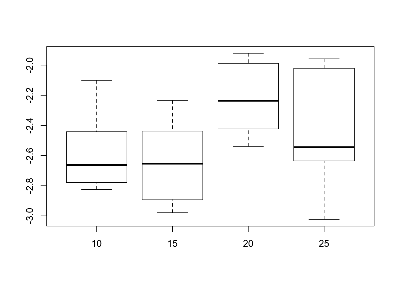

From the boxplots, it seems that LGWEIGHT increases with temperature. Also, the variance of LGWEIGHT seems to increase a little with temperature.

Analysis plan

Since we have a continous outcome and one categorical variable, we can analyse this with ANOVA (or equivalently: simple linear regression). We can treat temperature as a continous variable, or as a categorical one. Since we expect a monotonous relationship on the range of tested temperatures, we will use it as a continous variable, as this keeps in the information that \(temp = 10 < 15 < 20 < 25\)

Crude analysis

fit <- lm(LGWEIGHT~TEMP, data = cobweb)
summary(fit)


Call:
lm(formula = LGWEIGHT ~ TEMP, data = cobweb)

Residuals:
     Min       1Q   Median       3Q      Max 
-0.68955 -0.21504 -0.03525  0.27801  0.49991 

Coefficients:
             Estimate Std. Error t value Pr(>|t|)    
(Intercept) -2.769883   0.178248 -15.539   <2e-16 ***
TEMP         0.017440   0.009537   1.829   0.0765 .  
---
Signif. codes:  0 '***' 0.001 '**' 0.01 '*' 0.05 '.' 0.1 ' ' 1

Residual standard error: 0.3111 on 33 degrees of freedom
Multiple R-squared:  0.092, Adjusted R-squared:  0.06449 
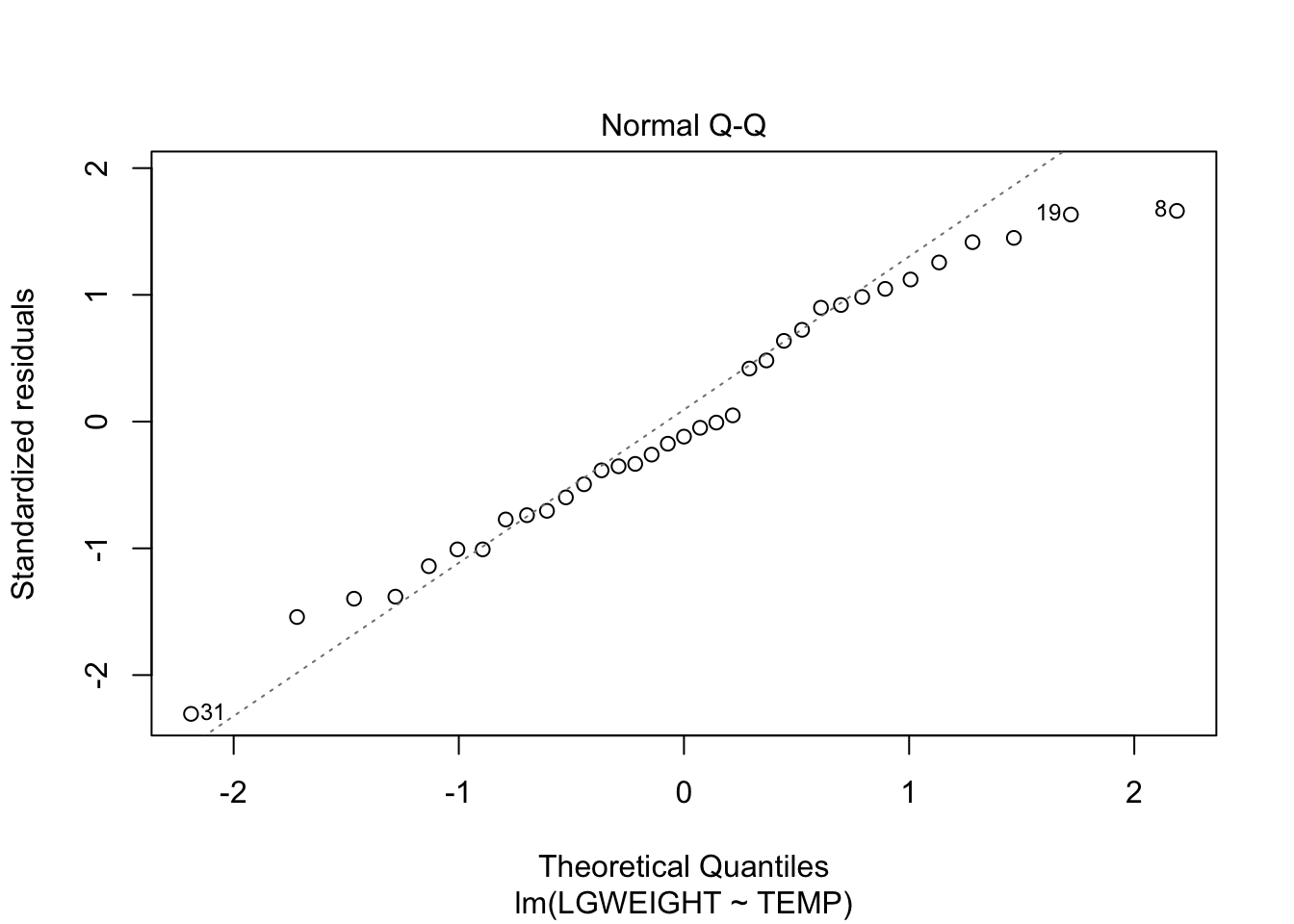
F-statistic: 3.344 on 1 and 33 DF,  p-value: 0.07651

plot(fit, which = c(1,2))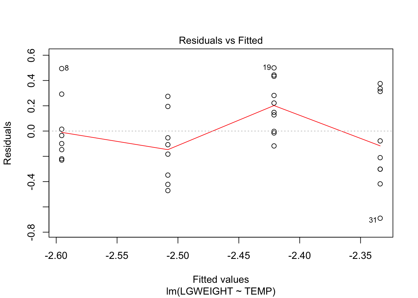

cor.test(~LGWEIGHT+TEMP, data = cobweb, method = "spearman")

Warning in cor.test.default(x = c(-2.81508, -2.74254, -2.69473, -2.58087, :
Cannot compute exact p-value with ties


    Spearman's rank correlation rho

data:  LGWEIGHT and TEMP
S = 4961.6, p-value = 0.07472
alternative hypothesis: true rho is not equal to 0
sample estimates:
      rho 
0.3050958

From the analysis, it looks like there is

fit_anova <- aov(LGWEIGHT~factor(TEMP), data = cobweb)
summary(fit_anova)

             Df Sum Sq Mean Sq F value Pr(>F)  
factor(TEMP)  3 0.9939  0.3313   4.068 0.0151 *
Residuals    31 2.5246  0.0814                 
---
Signif. codes:  0 '***' 0.001 '**' 0.01 '*' 0.05 '.' 0.1 ' ' 1

TukeyHSD(fit_anova)

  Tukey multiple comparisons of means
    95% family-wise confidence level

Fit: aov(formula = LGWEIGHT ~ factor(TEMP), data = cobweb)

$`factor(TEMP)`
            diff          lwr       upr     p adj
15-10 -0.0611375 -0.448403316 0.3261283 0.9731521
20-10  0.3676185  0.000225888 0.7350111 0.0498135
25-10  0.1444531 -0.231901669 0.5208078 0.7265602
20-15  0.4287560  0.061363388 0.7961486 0.0171924
25-15  0.2055906 -0.170764169 0.5819453 0.4597789
25-20 -0.2231654 -0.579038171 0.1327073 0.3398488

Multiple regression

Interpretation of results

Conclusions

Case Study 5, immediate vs sustained release

Immediate release medications quickly liberate their drug content into the body, with the maximum concentration reached in a short time followed by a rapid decline in concentration. Sustained release medications, on the other hand, take longer to reach maximum concentration in the body and stay active for longer periods of time.

A study of two such pain relief medications compared immediate release codeine (IRC) with sustained release codeine (SRC). Thirteen healthy patients were randomly assigned to one of the two types of codeine and treated for 2.5 days. After a 7-day wash-out period, the same patients were given the other type of codeine. Measurements include the maximum concentration in ng/mL, the time to maximum concentration in hours, the total amount of drug available over the life of the treatment in (ng*mL)/hr and the age of the patient. These data are shown below (see also the file codeine.sav or codeine.RData.

Concentration   Time    Total amount

Age IRC SRC IRC SRC IRC SRC 33 181.8 195.7 0.5 2.0 1091.3 1308.5 40 466.9 167.0 1.0 3.0 1064.5 1494.2 41 136.0 217.3 0.5 3.0 1281.1 1382.2 43 221.3 375.7 1.5 4.5 1921.4 1978.3 25 195.1 285.7 0.5 2.0 1649.9 2004.6 30 112.7 177.2 1.0 2.0 1423.6 * 24 84.2 220.3 2.0 1.5 1308.4 1211.1 44 78.5 243.5 1.0 3.0 1192.1 1002.4 42 85.9 141.6 1.5 1.5 766.2 866.6 33 85.3 127.2 2.0 4.5 978.6 1345.8 38 217.2 345.2 0.5 1.5 1618.9 979.2 39 49.7 112.1 1.5 1.0 582.9 576.3 43 190.0 223.4 0.5 1.0 972.1 999.1

The research questions are: are there any differences on these three parameters between immediate release codeine and sustained release codeine? Are these differences dependent on age?

Research objective

Assume random order.

Research question

Variables of interest

determinant:
outcome:
possible confounders:

Data exploration

load(epistats::fromParentDir("data/codeine.RData"))
str(codeine)

List of 7
 $ AGE : num [1:13] 33 40 41 43 25 30 24 44 42 33 ...
 $ CIRC: num [1:13] 182 467 136 221 195 ...
 $ CSRC: num [1:13] 196 167 217 376 286 ...
 $ TIRC: num [1:13] 0.5 1 0.5 1.5 0.5 1 2 1 1.5 2 ...
 $ TSRC: num [1:13] 2 3 3 4.5 2 2 1.5 3 1.5 4.5 ...
 $ AIRC: num [1:13] 1091 1064 1281 1921 1650 ...
 $ ASRC: num [1:13] 1308 1494 1382 1978 2005 ...
 - attr(*, "label.table")=List of 7
  ..$ AGE : NULL
  ..$ CIRC: NULL
  ..$ CSRC: NULL
  ..$ TIRC: NULL
  ..$ TSRC: NULL
  ..$ AIRC: NULL
  ..$ ASRC: NULL

codeine <- as.data.frame(codeine)

Data curation

Melt into easier format

codein_melted <- data.table::melt(codeine, id.vars = "AGE")

Pairs plot

Analysis plan

We will use the parametric tests. Too little data to check assumptions, too little data for power for non-parametric tests.

Crude analysis

t.test(codeine)


    One Sample t-test

data:  codeine
t = 6.7874, df = 89, p-value = 1.227e-09
alternative hypothesis: true mean is not equal to 0
95 percent confidence interval:
 286.4803 523.6375
sample estimates:
mean of x 
 405.0589

Multiple regression

Dependent on age:

Difference ~ age (dependent -> regression, associated -> correlation)

Interpretation of results

Conclusions

General structure

(for later take heading levels up 1 step) #### Case description

Research objective

Research question

Variables of interest

determinant:
outcome:
possible confounders:

Data exploration

Data curation

Pairs plot

Analysis plan

Crude analysis

Multiple regression

Interpretation of results

Conclusions

Session information

sessionInfo()

R version 3.3.2 (2016-10-31)
Platform: x86_64-apple-darwin13.4.0 (64-bit)
Running under: macOS Sierra 10.12.6

locale:
[1] en_US.UTF-8/en_US.UTF-8/en_US.UTF-8/C/en_US.UTF-8/en_US.UTF-8

attached base packages:
[1] stats     graphics  grDevices utils     datasets  methods   base     

other attached packages:
[1] survival_2.41-3 ggplot2_2.2.1   bindrcpp_0.2    dplyr_0.7.4    
[5] GGally_1.3.1   

loaded via a namespace (and not attached):
 [1] Rcpp_0.12.14       nloptr_1.0.4       RColorBrewer_1.1-2
 [4] git2r_0.20.0       plyr_1.8.4         bindr_0.1         
 [7] epistats_0.1.0     tools_3.3.2        lme4_1.1-13       
[10] digest_0.6.13      nlme_3.1-131       evaluate_0.10.1   
[13] tibble_1.3.4       gtable_0.2.0       lattice_0.20-35   
[16] mgcv_1.8-17        pkgconfig_2.0.1    rlang_0.1.6       
[19] Matrix_1.2-10      parallel_3.3.2     yaml_2.1.16       
[22] SparseM_1.77       stringr_1.2.0      knitr_1.18        
[25] MatrixModels_0.4-1 nnet_7.3-12        rprojroot_1.2     
[28] lmtest_0.9-35      grid_3.3.2         data.table_1.10.4 
[31] reshape_0.8.6      glue_1.2.0         R6_2.2.2          
[34] rmarkdown_1.8      minqa_1.2.4        car_2.1-5         
[37] reshape2_1.4.2     magrittr_1.5       MASS_7.3-47       
[40] splines_3.3.2      backports_1.1.0    scales_0.4.1      
[43] htmltools_0.3.6    pbkrtest_0.4-7     assertthat_0.2.0  
[46] colorspace_1.3-2   quantreg_5.33      labeling_0.3      
[49] stringi_1.1.6      lazyeval_0.2.0     munsell_0.4.3     
[52] zoo_1.8-0

This R Markdown site was created with workflowr

Case Studies - not finished

Wouter van Amsterdam

2017-11-10

NB Not finished

Instructions

The Case Studies

Case Study 1: fruitflies

Research objective

Variables of interest

Data exploration

Data curation

Pairs plot

Analysis plan

Interpretation of results

Crude analysis

Multiple regression

Conclusions

Case Study 2, Heroin rehab clinic

Research objective

Research question

Variables of interest

Data exploration

Data curation

Pairs plot

Analysis plan

Crude analysis

Multiple regression

Interpretation of results

Conclusions

Case Study 3, Maternal mortality rates

Research objective

Research question

Variables of interest

Data exploration

Data curation

Pairs plot

Analysis plan

Crude analysis

Multiple regression

Interpretation of results

Conclusions

Case Study 4, Spider web

Research objective

Research question

Variables of interest

Data exploration

Data curation

Pairs plot

Analysis plan

Crude analysis

Multiple regression

Interpretation of results

Conclusions

Case Study 5, immediate vs sustained release

Research objective

Research question

Variables of interest

Data exploration

Data curation

Pairs plot

Analysis plan

Crude analysis

Multiple regression

Interpretation of results

Conclusions

General structure

Research objective

Research question

Variables of interest

Data exploration

Data curation

Pairs plot

Analysis plan

Crude analysis

Multiple regression

Interpretation of results

Conclusions

Session information