Presentation lung cancer survival prediction

Last updated: 2018-04-20

Code version: e96adb1

Setup R environment

library(dplyr)
library(data.table)
library(magrittr)
library(purrr)
library(here) # for tracking working directory
library(ggplot2)
library(epistats)
library(broom)
library(survival)

Get Data

lc <- read.csv(here("data", "lungca.csv"))

cont_vars <- c("age", "Karn.phys", "Karn.pt", "wtloss")

lc %<>% 
  mutate(status = status - 1,
         sex = factor(sex, levels = c("1", "2"), labels = c("male", "female")),
         wtloss = 0.453592 * wtloss,
         ECOG.phys = factor(ifelse(ECOG.phys == "3", "2", ECOG.phys)),
         ECOG.phys = factor(ECOG.phys, levels = c("0", "1", "2"), 
                            labels = c("0", "1", "2-3")))
         # age = age - mean(age))


str(lc)

'data.frame':   167 obs. of  10 variables:
 $ center   : int  3 5 12 7 11 1 7 6 12 22 ...
 $ time     : int  455 210 1022 310 361 218 166 170 567 613 ...
 $ status   : num  1 1 0 1 1 1 1 1 1 1 ...
 $ age      : int  68 57 74 68 71 53 61 57 57 70 ...
 $ sex      : Factor w/ 2 levels "male","female": 1 1 1 2 2 1 1 1 1 1 ...
 $ ECOG.phys: Factor w/ 3 levels "0","1","2-3": 1 2 2 3 3 2 3 2 2 2 ...
 $ Karn.phys: int  90 90 50 70 60 70 70 80 80 90 ...
 $ Karn.pt  : int  90 60 80 60 80 80 70 80 70 100 ...
 $ calories : int  1225 1150 513 384 538 825 271 1025 2600 1150 ...
 $ wtloss   : num  6.804 4.99 0 4.536 0.454 ...

summary(lc)

     center           time            status            age       
 Min.   : 1.00   Min.   :   5.0   Min.   :0.0000   Min.   :39.00  
 1st Qu.: 3.00   1st Qu.: 174.5   1st Qu.:0.0000   1st Qu.:57.00  
 Median :11.00   Median : 268.0   Median :1.0000   Median :64.00  
 Mean   :10.71   Mean   : 309.9   Mean   :0.7186   Mean   :62.57  
 3rd Qu.:15.00   3rd Qu.: 419.5   3rd Qu.:1.0000   3rd Qu.:70.00  
 Max.   :32.00   Max.   :1022.0   Max.   :1.0000   Max.   :82.00  
     sex      ECOG.phys   Karn.phys         Karn.pt          calories     
 male  :103   0  :47    Min.   : 50.00   Min.   : 30.00   Min.   :  96.0  
 female: 64   1  :81    1st Qu.: 70.00   1st Qu.: 70.00   1st Qu.: 619.0  
              2-3:39    Median : 80.00   Median : 80.00   Median : 975.0  
                        Mean   : 82.04   Mean   : 79.58   Mean   : 929.1  
                        3rd Qu.: 90.00   3rd Qu.: 90.00   3rd Qu.:1162.5  
                        Max.   :100.00   Max.   :100.00   Max.   :2600.0  
     wtloss       
 Min.   :-10.886  
 1st Qu.:  0.000  
 Median :  3.175  
 Mean   :  4.408  
 3rd Qu.:  6.804  
 Max.   : 30.844

nna(lc)

   center      time    status       age       sex ECOG.phys Karn.phys 
        0         0         0         0         0         0         0 
  Karn.pt  calories    wtloss 
        0         0         0

table(lc$ECOG.phys, lc$sex)

     
      male female
  0     28     19
  1     52     29
  2-3   23     16

lc %>%
  data.table::melt(measure.vars = cont_vars) %>% 
  ggplot(aes(x = value)) + 
  geom_histogram() + 
  facet_grid(sex~variable, scales = "free_x") + 
  theme_minimal()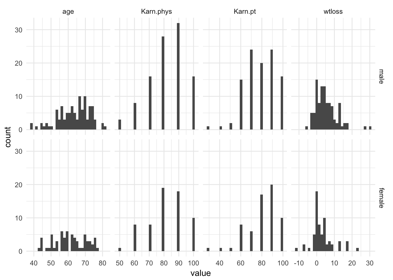

Recode Karnophsky as factors

factor_vars <- c("center", "sex", "ECOG.phys", "Karn.phys", "Karn.pt")
lc %<>%
  mutate_at(vars(factor_vars), funs(as.factor))

lc %>%
  ggplot(aes(x = calories, y = wtloss)) + 
  geom_point() + theme_minimal()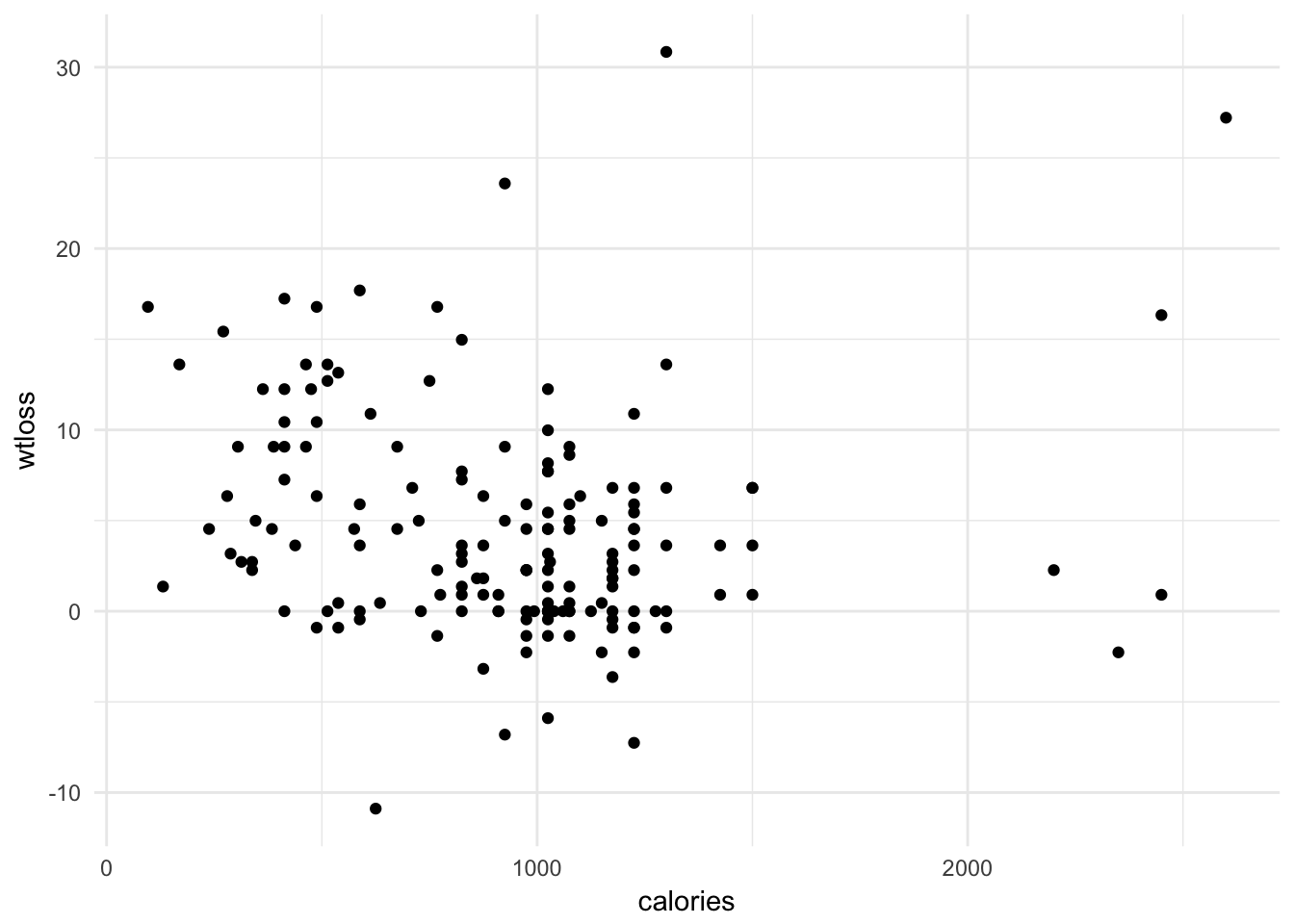

lc %>%
  mutate(
    wt_loss_ratio = wtloss / calories
  ) %>%
  ggplot(aes(x = wt_loss_ratio)) + 
  geom_histogram()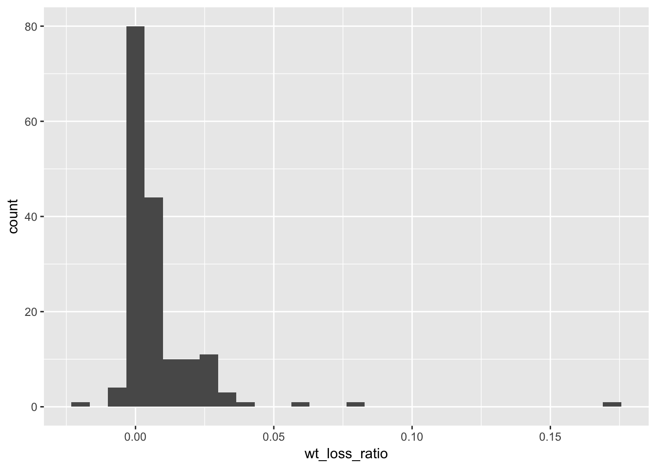

Overview of survival

require(ggfortify)
surv_plot <- lc %>%
  survfit(Surv(time / 365, status) ~ 1, data = .) %>%
  autoplot() + theme_minimal() + 
  labs(x = "Time (years)",
       y = "Survival probability") + 
  ggtitle("Overview of survival (Kaplan-Meier estimate)")
surv_plot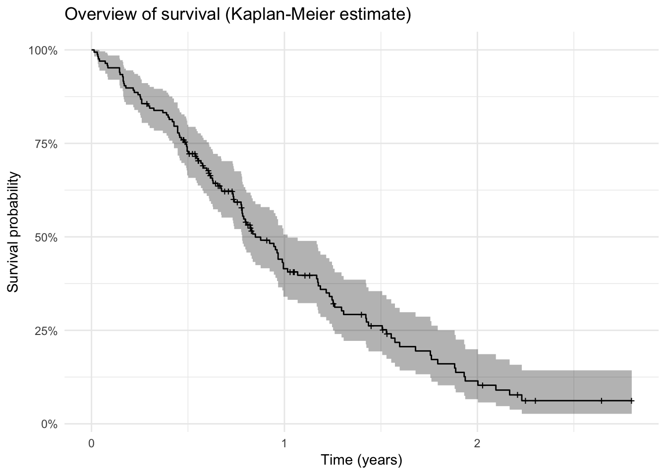

survfit1 <- survfit(Surv(time, status) ~ 1, data = lc)
print(survfit1)

Call: survfit(formula = Surv(time, status) ~ 1, data = lc)

      n  events  median 0.95LCL 0.95UCL 
    167     120     310     285     371

require(ggfortify)
lc %>%
  mutate(dummy_variable = T,
         status = factor(status, levels = c(0, 1), labels = c("censored", "deceased"))) %>%
  survfit(Surv(time / 365, dummy_variable) ~ status, data = .) %>%
  autoplot() + theme_minimal()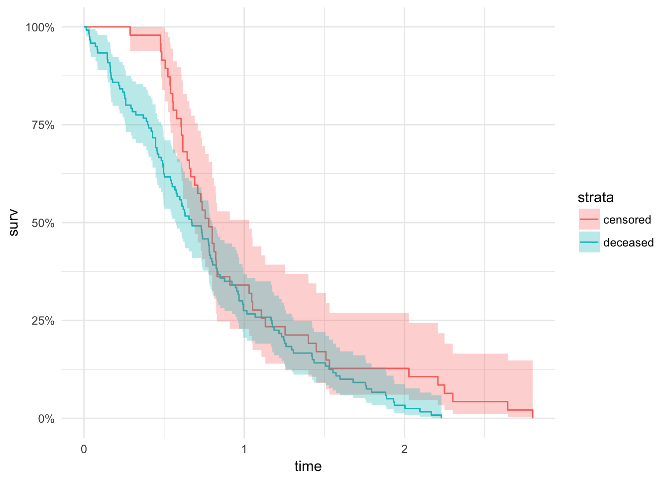

lc %>%
  coxph(Surv(time, status) ~ age + sex + ECOG.phys + Karn.phys + Karn.pt + calories + wtloss, 
        data = .) %>%
  summary()

Call:
coxph(formula = Surv(time, status) ~ age + sex + ECOG.phys + 
    Karn.phys + Karn.pt + calories + wtloss, data = .)

  n= 167, number of events= 120 

                   coef  exp(coef)   se(coef)      z Pr(>|z|)   
age           6.272e-03  1.006e+00  1.205e-02  0.520  0.60286   
sexfemale    -6.211e-01  5.373e-01  2.146e-01 -2.894  0.00381 **
ECOG.phys1    6.387e-01  1.894e+00  3.527e-01  1.811  0.07018 . 
ECOG.phys2-3  1.357e+00  3.885e+00  5.451e-01  2.490  0.01278 * 
Karn.phys60   1.101e+00  3.007e+00  6.825e-01  1.613  0.10670   
Karn.phys70   1.025e+00  2.787e+00  6.556e-01  1.564  0.11792   
Karn.phys80   1.200e+00  3.321e+00  6.681e-01  1.796  0.07244 . 
Karn.phys90   1.341e+00  3.822e+00  6.859e-01  1.955  0.05058 . 
Karn.phys100  1.484e+00  4.411e+00  7.743e-01  1.917  0.05528 . 
Karn.pt40    -3.821e-01  6.824e-01  1.521e+00 -0.251  0.80158   
Karn.pt50     7.358e-01  2.087e+00  1.216e+00  0.605  0.54524   
Karn.pt60     1.340e-01  1.143e+00  1.042e+00  0.129  0.89773   
Karn.pt70    -1.180e-01  8.887e-01  1.078e+00 -0.109  0.91283   
Karn.pt80    -2.206e-01  8.020e-01  1.086e+00 -0.203  0.83906   
Karn.pt90    -1.580e-02  9.843e-01  1.082e+00 -0.015  0.98835   
Karn.pt100   -5.112e-01  5.998e-01  1.105e+00 -0.463  0.64366   
calories     -5.387e-05  9.999e-01  2.839e-04 -0.190  0.84952   
wtloss       -3.021e-02  9.702e-01  1.831e-02 -1.650  0.09903 . 
---
Signif. codes:  0 '***' 0.001 '**' 0.01 '*' 0.05 '.' 0.1 ' ' 1

             exp(coef) exp(-coef) lower .95 upper .95
age             1.0063     0.9937   0.98280    1.0303
sexfemale       0.5373     1.8610   0.35281    0.8184
ECOG.phys1      1.8940     0.5280   0.94873    3.7810
ECOG.phys2-3    3.8849     0.2574   1.33485   11.3067
Karn.phys60     3.0072     0.3325   0.78925   11.4580
Karn.phys70     2.7874     0.3588   0.77114   10.0752
Karn.phys80     3.3208     0.3011   0.89644   12.3015
Karn.phys90     3.8222     0.2616   0.99660   14.6594
Karn.phys100    4.4111     0.2267   0.96701   20.1219
Karn.pt40       0.6824     1.4654   0.03465   13.4403
Karn.pt50       2.0871     0.4791   0.19241   22.6384
Karn.pt60       1.1434     0.8746   0.14819    8.8218
Karn.pt70       0.8887     1.1252   0.10745    7.3502
Karn.pt80       0.8020     1.2468   0.09543    6.7411
Karn.pt90       0.9843     1.0159   0.11805    8.2077
Karn.pt100      0.5998     1.6673   0.06877    5.2312
calories        0.9999     1.0001   0.99939    1.0005
wtloss          0.9702     1.0307   0.93603    1.0057

Concordance= 0.662  (se = 0.031 )
Rsquare= 0.182   (max possible= 0.998 )
Likelihood ratio test= 33.53  on 18 df,   p=0.01437
Wald test            = 33.29  on 18 df,   p=0.01539
Score (logrank) test = 35.97  on 18 df,   p=0.007125

Model with random intercept per center

Random slopes make no sense -> why different effect of age in different centers?

fit1 <- coxph(Surv(time, status) ~ age + sex + ECOG.phys + Karn.phys + Karn.pt + calories * wtloss + frailty(center, dist = "gauss"),
        data = lc)
# summary(fit)

fit2 <- coxph(Surv(time, status) ~ age + sex + ECOG.phys + Karn.phys + Karn.pt + calories * wtloss,
        data = lc)

fits <- list(with_random_full = fit1, no_random_full = fit2)

map_df(fits, extractAIC)

# A tibble: 2 x 2
  with_random_full no_random_full
             <dbl>          <dbl>
1             23.9           19.0
2           1014           1021

extractAIC(fit1)

[1]   23.91509 1014.17005

extractAIC(fit2)

[1]   19.000 1020.647

anova(fit1, fit2, test = "Chisq")

Analysis of Deviance Table
 Cox model: response is  Surv(time, status)
 Model 1: ~ age + sex + ECOG.phys + Karn.phys + Karn.pt + calories * wtloss + frailty(center, dist = "gauss")
 Model 2: ~ age + sex + ECOG.phys + Karn.phys + Karn.pt + calories * wtloss
   loglik  Chisq     Df P(>|Chi|)   
1 -483.17                           
2 -491.32 16.307 4.9151   0.00564 **
---
Signif. codes:  0 '***' 0.001 '**' 0.01 '*' 0.05 '.' 0.1 ' ' 1

With manual likelihood-ratio test for chi-square distribution with 1 degree of freedom

pchisq(2*(logLik(fit1) - logLik(fit2)), df = 1, lower.tail = F)

'log Lik.' 5.38541e-05 (df=0.9761468)

Follow LRT the model with random intercept per center is better.

Use this random part, now reduce fixed part.

fit_full <- coxph(Surv(time, status) ~ age + sex + ECOG.phys + Karn.phys + Karn.pt + calories * wtloss + frailty(center, dist = "gauss"), data = lc)

fit <- fit_full
drop1(fit, test = "Chisq")

Single term deletions

Model:
Surv(time, status) ~ age + sex + ECOG.phys + Karn.phys + Karn.pt + 
    calories * wtloss + frailty(center, dist = "gauss")
                                     Df    AIC     LRT Pr(>Chi)   
<none>                                  1014.2                    
age                             0.84864 1012.4 -0.1119 1.000000   
sex                             2.69586 1024.0 15.2547 0.001155 **
ECOG.phys                       1.32255 1016.3  4.7459 0.045981 * 
Karn.phys                       5.23149 1010.7  7.0146 0.241562   
Karn.pt                         6.35830 1004.7  3.2178 0.814319   
frailty(center, dist = "gauss") 4.91509 1020.6 16.3074 0.005640 **
calories:wtloss                 1.00408 1012.4  0.2284 0.634434   
---
Signif. codes:  0 '***' 0.001 '**' 0.01 '*' 0.05 '.' 0.1 ' ' 1

fit <- coxph(Surv(time, status) ~ sex + ECOG.phys + Karn.phys + Karn.pt + calories * wtloss + frailty(center, dist = "gauss"),
        data = lc)
drop1(fit, test = "Chisq")

Single term deletions

Model:
Surv(time, status) ~ sex + ECOG.phys + Karn.phys + Karn.pt + 
    calories * wtloss + frailty(center, dist = "gauss")
                                     Df    AIC     LRT Pr(>Chi)   
<none>                                  1012.4                    
sex                             2.71446 1022.4 15.4992 0.001049 **
ECOG.phys                       1.39257 1014.5  4.9108 0.045759 * 
Karn.phys                       5.34558 1008.8  7.1333 0.243242   
Karn.pt                         6.26163 1003.0  3.1719 0.811303   
frailty(center, dist = "gauss") 5.06645 1018.9 16.6657 0.005450 **
calories:wtloss                 0.97932 1010.6  0.2180 0.631965   
---
Signif. codes:  0 '***' 0.001 '**' 0.01 '*' 0.05 '.' 0.1 ' ' 1

fit <- coxph(Surv(time, status) ~ sex + ECOG.phys + Karn.phys + calories * wtloss + frailty(center, dist = "gauss"),
        data = lc)
drop1(fit, test = "Chisq")

Single term deletions

Model:
Surv(time, status) ~ sex + ECOG.phys + Karn.phys + calories * 
    wtloss + frailty(center, dist = "gauss")
                                     Df    AIC     LRT  Pr(>Chi)    
<none>                                  1003.0                      
sex                             2.61157 1014.6 16.7801 0.0005019 ***
ECOG.phys                       2.01604 1009.2 10.2417 0.0060855 ** 
Karn.phys                       5.64572 1001.5  9.8126 0.1125923    
frailty(center, dist = "gauss") 5.80483 1009.6 18.2374 0.0049296 ** 
calories:wtloss                 0.94795 1001.3  0.1821 0.6477098    
---
Signif. codes:  0 '***' 0.001 '**' 0.01 '*' 0.05 '.' 0.1 ' ' 1

fit <- coxph(Surv(time, status) ~ sex + ECOG.phys + Karn.phys + calories + wtloss + frailty(center, dist = "gauss"),
        data = lc)
drop1(fit, test = "Chisq")

Single term deletions

Model:
Surv(time, status) ~ sex + ECOG.phys + Karn.phys + calories + 
    wtloss + frailty(center, dist = "gauss")
                                    Df    AIC     LRT  Pr(>Chi)    
<none>                                 1001.3                      
sex                             2.6093 1012.9 16.7953 0.0004968 ***
ECOG.phys                       2.0940 1007.5 10.4420 0.0060347 ** 
Karn.phys                       5.7320 1000.2 10.3679 0.0966516 .  
calories                        1.2941 1000.1  1.3760 0.3201357    
wtloss                          1.5644 1004.2  6.0541 0.0303939 *  
frailty(center, dist = "gauss") 5.8569 1007.8 18.1768 0.0052451 ** 
---
Signif. codes:  0 '***' 0.001 '**' 0.01 '*' 0.05 '.' 0.1 ' ' 1

fit <- coxph(Surv(time, status) ~ sex + ECOG.phys + Karn.phys + wtloss + frailty(center, dist = "gauss"),
        data = lc)
drop1(fit, test = "Chisq")

Single term deletions

Model:
Surv(time, status) ~ sex + ECOG.phys + Karn.phys + wtloss + frailty(center, 
    dist = "gauss")
                                    Df     AIC     LRT  Pr(>Chi)    
<none>                                 1000.08                      
sex                             2.3324 1010.94 15.5180 0.0006593 ***
ECOG.phys                       2.3676 1006.90 11.5541 0.0047662 ** 
Karn.phys                       5.5511  998.46  9.4831 0.1207032    
wtloss                          1.7026 1003.14  6.4606 0.0288310 *  
frailty(center, dist = "gauss") 5.5628 1005.89 16.9309 0.0070480 ** 
---
Signif. codes:  0 '***' 0.001 '**' 0.01 '*' 0.05 '.' 0.1 ' ' 1

fit <- coxph(Surv(time, status) ~ sex + ECOG.phys + wtloss + frailty(center, dist = "gauss"),
        data = lc)
drop1(fit, test = "Chisq")

Single term deletions

Model:
Surv(time, status) ~ sex + ECOG.phys + wtloss + frailty(center, 
    dist = "gauss")
                                    Df     AIC     LRT  Pr(>Chi)    
<none>                                  998.46                      
sex                             1.8785 1005.85 11.1391 0.0032752 ** 
ECOG.phys                       6.7385 1013.96 28.9683 0.0001179 ***
wtloss                          1.2017  999.66  3.5979 0.0758057 .  
frailty(center, dist = "gauss") 5.0117 1001.90 13.4614 0.0195731 *  
---
Signif. codes:  0 '***' 0.001 '**' 0.01 '*' 0.05 '.' 0.1 ' ' 1

fit <- coxph(Surv(time, status) ~ sex + ECOG.phys + frailty(center, dist = "gauss"),
        data = lc)
drop1(fit, test = "Chisq")

Single term deletions

Model:
Surv(time, status) ~ sex + ECOG.phys + frailty(center, dist = "gauss")
                                    Df     AIC     LRT  Pr(>Chi)    
<none>                                  999.66                      
sex                             1.5970 1005.44  8.9712 0.0068833 ** 
ECOG.phys                       6.6708 1011.98 25.6673 0.0004465 ***
frailty(center, dist = "gauss") 4.8100 1002.65 12.6151 0.0240372 *  
---
Signif. codes:  0 '***' 0.001 '**' 0.01 '*' 0.05 '.' 0.1 ' ' 1

fit_final <- coxph(Surv(time, status) ~ sex + ECOG.phys + frailty(center, dist = "gauss"), data = lc)
summary(fit_final)

Call:
coxph(formula = Surv(time, status) ~ sex + ECOG.phys + frailty(center, 
    dist = "gauss"), data = lc)

  n= 167, number of events= 120 

                          coef    se(coef) se2    Chisq DF   p      
sexfemale                 -0.5269 0.1986   0.1973  7.04 1.00 8.0e-03
ECOG.phys1                 0.3268 0.2391   0.2350  1.87 1.00 1.7e-01
ECOG.phys2-3               1.0598 0.2693   0.2628 15.49 1.00 8.3e-05
frailty(center, dist = "g                          7.71 4.92 1.7e-01

             exp(coef) exp(-coef) lower .95 upper .95
sexfemale       0.5904     1.6937    0.4001    0.8714
ECOG.phys1      1.3866     0.7212    0.8678    2.2156
ECOG.phys2-3    2.8859     0.3465    1.7023    4.8925

Iterations: 8 outer, 30 Newton-Raphson
     Variance of random effect= 0.07332914 
Degrees of freedom for terms= 1.0 1.9 4.9 
Concordance= 0.674  (se = 0.031 )
Likelihood ratio test= 32.19  on 7.81 df,   p=7.379e-05

knitr::kable(extract_RR(fit_final))

	estimate	ci_low	ci_high
sexfemale	0.5904203	0.2011851	0.9796554
ECOG.phys1	1.3865878	0.9179148	1.8552608
ECOG.phys2-3	2.8858958	2.3580244	3.4137673

cox.zph(fit_final)

                 rho chisq      p
sexfemale     0.1074 1.357 0.2441
ECOG.phys1   -0.0522 0.341 0.5594
ECOG.phys2-3 -0.1836 4.165 0.0413
GLOBAL            NA 6.115 0.1061

lc %<>% mutate(lp = fit_final$linear.predictors)
lc %>%
  mutate(lp_quantile = quant(lp, n.tiles = 3, label = "risk group ")) %>%
  survfit(Surv(time / 365, status) ~ lp_quantile, data = .) %>%
  autoplot() + theme_minimal() +
  labs(x = "Time (years)",
       y = "Survival probability") + 
  ggtitle("Overview of survival (Kaplan-Meier estimate)", "strata by terciles of linear predictor")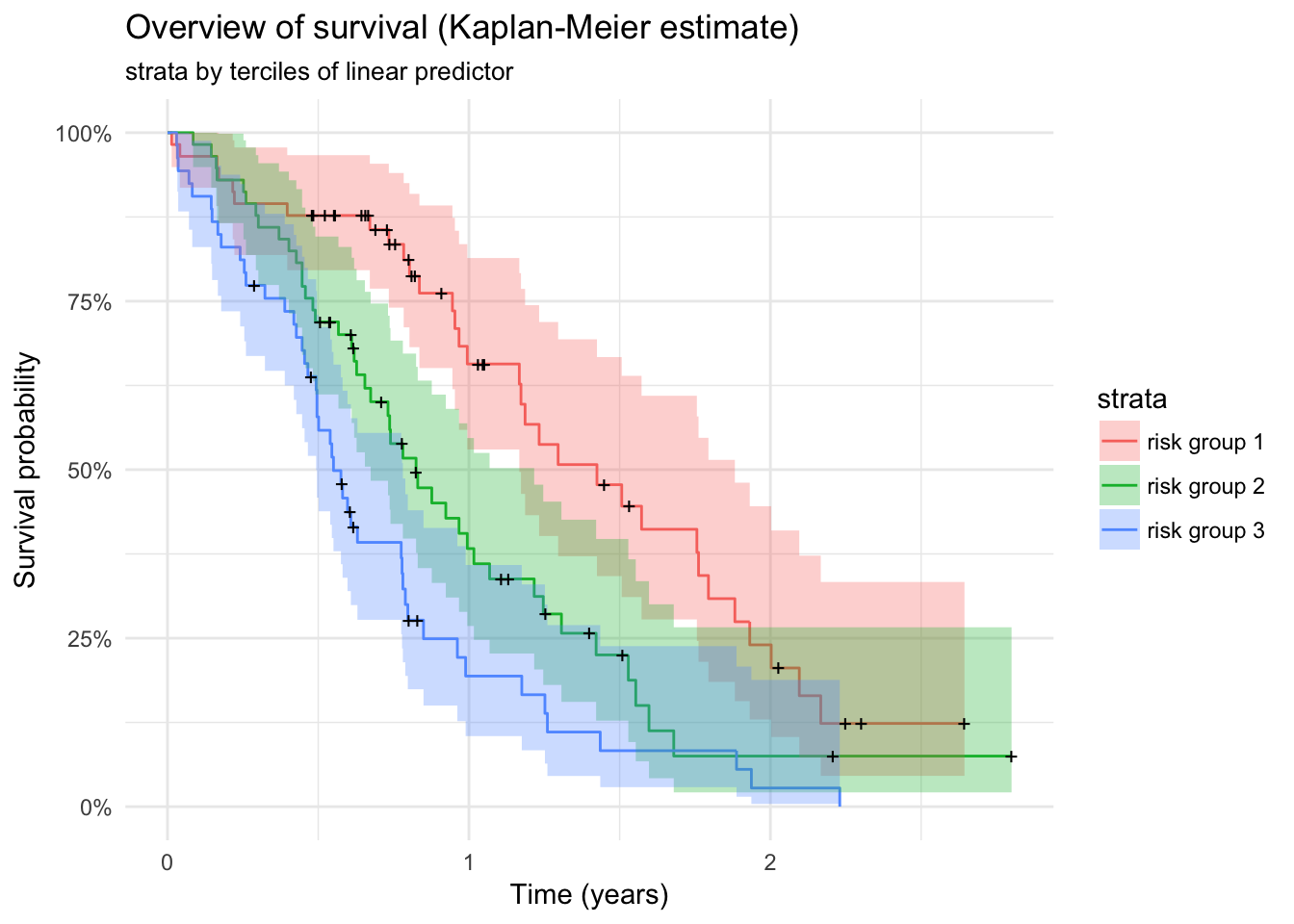

lc %>%
  survfit(Surv(time / 365, status) ~ sex, data = .) %>%
  autoplot() + theme_minimal() +
  labs(x = "Time (years)",
       y = "Survival probability") + 
  ggtitle("Overview of survival (Kaplan-Meier estimate)", "strata by sex")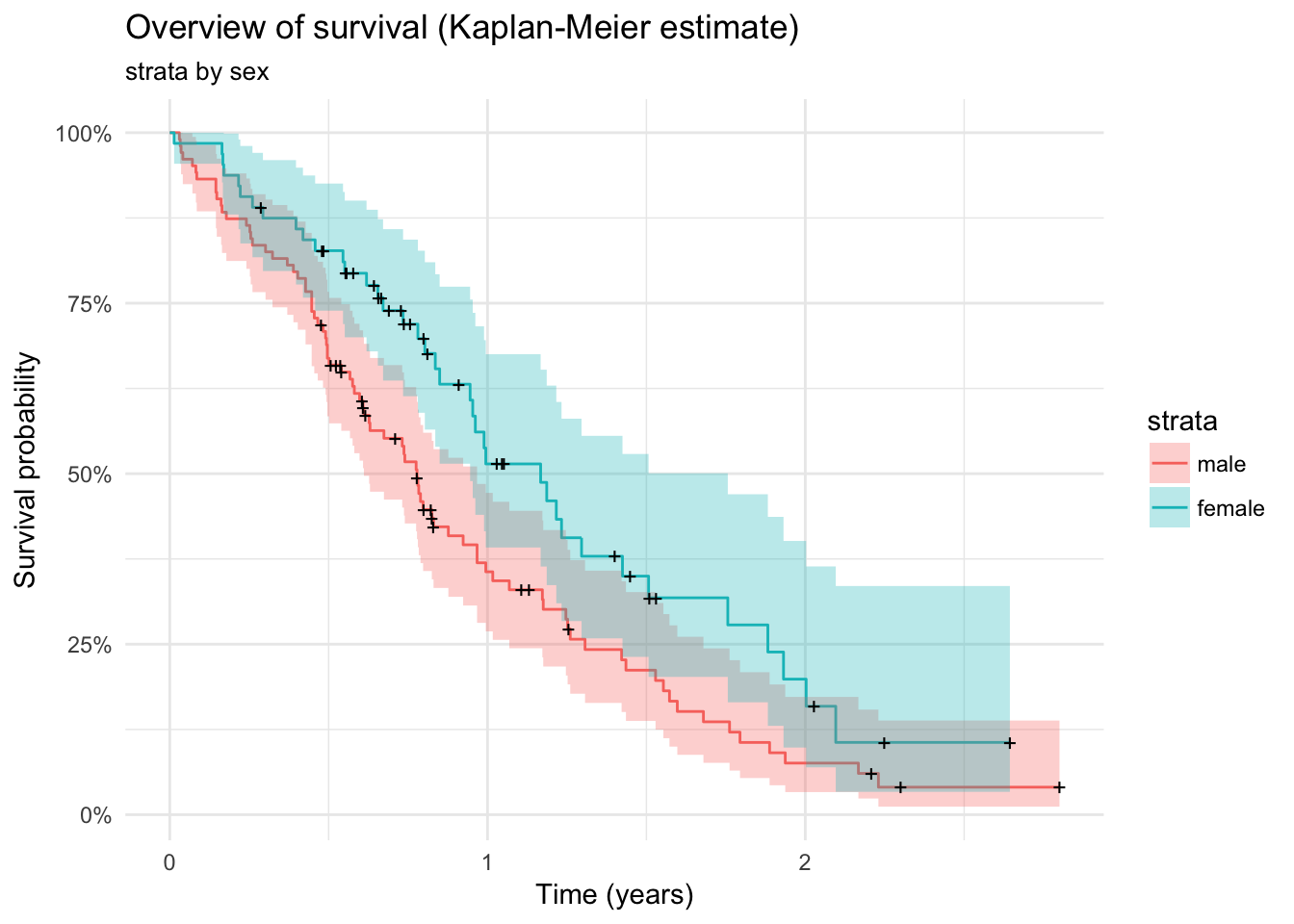

lc %>%
  survfit(Surv(time / 365, status) ~ ECOG.phys, data = .) %>% 
  autoplot() + theme_minimal() +
  labs(x = "Time (years)",
       y = "Survival probability") +
  ggtitle("Overview of survival (Kaplan-Meier estimate)",
          "strata by ECOG performance score")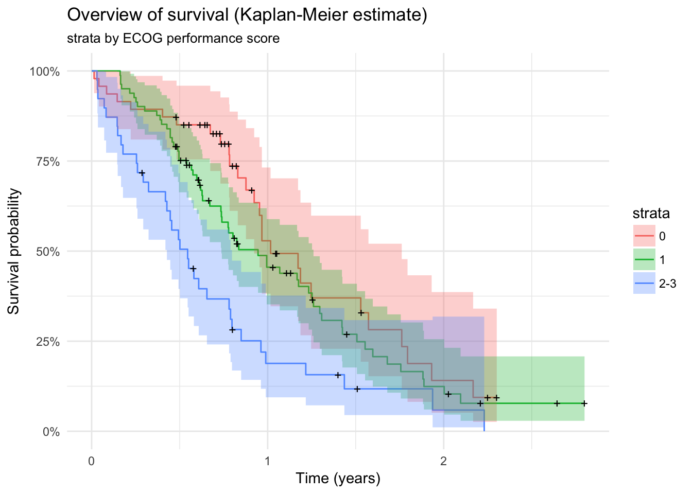

fit_sex <- coxph(Surv(time, status)~ strata(sex) + ECOG.phys + frailty(center, "gauss"), data = lc)
plot(survfit(fit_sex), fun = "cloglog",
     main = "c-loglog plot for final model stratified by sex",
     col = c("blue", "red"))
legend("topleft", c("male", "female"), col = c("blue", "red"), lty = 1)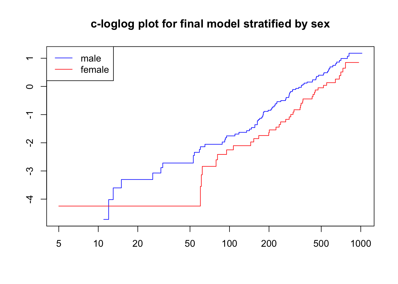

fit_ecog <- coxph(Surv(time, status)~ sex + strata(ECOG.phys) + frailty(center, "gauss"), data = lc)
plot(survfit(fit_ecog), fun = "cloglog", col = c("green", "blue", "red"),
     main = "c-loglog plot for final model stratified by ECOG performance status")
legend("topleft", legend = c("0", "1", "2-3"), lty = 1, col = c("green", "blue", "red"))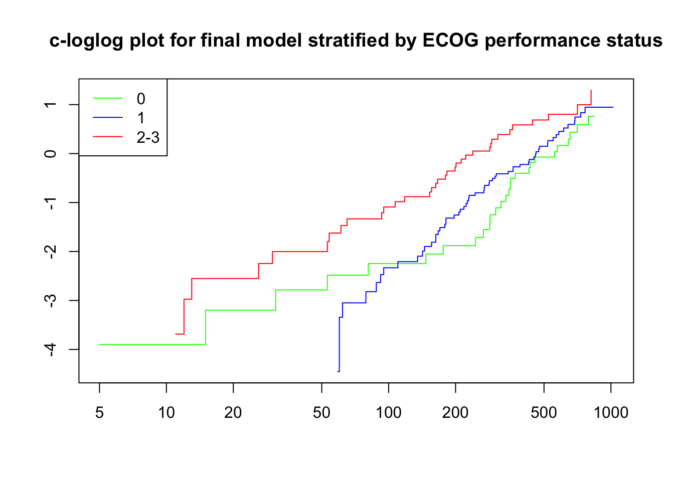

Session information

sessionInfo()

R version 3.4.3 (2017-11-30)
Platform: x86_64-apple-darwin15.6.0 (64-bit)
Running under: macOS Sierra 10.12.6

Matrix products: default
BLAS: /Library/Frameworks/R.framework/Versions/3.4/Resources/lib/libRblas.0.dylib
LAPACK: /Library/Frameworks/R.framework/Versions/3.4/Resources/lib/libRlapack.dylib

locale:
[1] en_US.UTF-8/en_US.UTF-8/en_US.UTF-8/C/en_US.UTF-8/en_US.UTF-8

attached base packages:
[1] stats     graphics  grDevices utils     datasets  methods   base     

other attached packages:
 [1] ggfortify_0.4.2     bindrcpp_0.2        survival_2.41-3    
 [4] broom_0.4.3         epistats_0.1.0      ggplot2_2.2.1      
 [7] here_0.1            purrr_0.2.4         magrittr_1.5       
[10] data.table_1.10.4-3 dplyr_0.7.4        

loaded via a namespace (and not attached):
 [1] Rcpp_0.12.15     highr_0.6        pillar_1.1.0     compiler_3.4.3  
 [5] git2r_0.21.0     plyr_1.8.4       bindr_0.1        tools_3.4.3     
 [9] digest_0.6.15    evaluate_0.10.1  tibble_1.4.2     gtable_0.2.0    
[13] nlme_3.1-131     lattice_0.20-35  pkgconfig_2.0.1  rlang_0.1.6     
[17] Matrix_1.2-12    psych_1.7.8      cli_1.0.0        parallel_3.4.3  
[21] yaml_2.1.16      gridExtra_2.3    stringr_1.2.0    knitr_1.19      
[25] rprojroot_1.3-2  grid_3.4.3       glue_1.2.0       R6_2.2.2        
[29] foreign_0.8-69   rmarkdown_1.8    reshape2_1.4.3   tidyr_0.8.0     
[33] splines_3.4.3    backports_1.1.2  scales_0.5.0     htmltools_0.3.6 
[37] mnormt_1.5-5     assertthat_0.2.0 colorspace_1.3-2 labeling_0.3    
[41] utf8_1.1.3       stringi_1.1.6    lazyeval_0.2.1   munsell_0.4.3   
[45] crayon_1.3.4

This R Markdown site was created with workflowr

Presentation lung cancer survival prediction

Wouter van Amsterdam

2018-04-20

Setup R environment

Get Data

Overview of survival

Session information