Assignments Modern Methods in Data Analysis, week 2

Last updated: 2018-04-16

Code version: 899ad0d

Setup

Load some packages

library(epistats) # contains 'fromParentDir' and other handy functions
library(magrittr) # for 'piping'  '%>%'
library(dplyr)    # for data mangling, selecting columns and filtering rows
library(ggplot2)  # awesome plotting library
library(stringr)  # for working with strings
library(purrr)    # for the 'map' function, which is an alternative for lapply, sapply, mapply, etc.

For installing packages, type install.packages(<package_name>), for instance: install.packages(dplyr)

epistats is only available from GitHub, and can be installed as follows:

install.packages(devtools) # when not installed already
devtools::install_github("vanAmsterdam/epistats")

Resampling

Most of the exercises below come from Moore and McCabe’s Introduction to Practical Statistics, (8th Ed) chapter 16; some have been adapted slightly. Note that for exercises 16.40 and further an R script with commands is available on Moodle. In the answers to the exercises, at the end of the current document, some extra explanation about the R commands is provided. You can also have a look at the following resource that explains most common bootstrap functions in R: http://www.statmethods.net/advstats/bootstrapping.html

Ex. 16.7 What is wrong?

Explain what is wrong with each of the following statements.

(a) The bootstrap distribution is created by resampling with replacement from the population.

It is created by resampling with replacement from the sample, not the population

(b) The bootstrap distribution is created by resampling without replacement from the original sample.

It is resampling with replacements

(c) When generating the resamples, it is best to use a sample size larger than the size of the original sample.

No, this will give falsly tight confidence bounds as you are simulating that you have gathered a lot of data, while you have only simulated data.

(d) The bootstrap distribution will be similar to the sampling distribution in shape, center, and spread.

The bootstrap distribution is centered around the the sample mean, with sample spread. These can be different from the population and thus different from the ‘true’ sampling distribution

Ex. 16.40 Confidence interval for the average IQ score.

The distribution of the 60 IQ test scores in IQ.txt is roughly Normal (make a histogram and normal QQ-plot to check this), and the sample size is large enough that we expect a Normal sampling distribution. We will compare confidence intervals for the population mean IQ μ based on this sample.

(a) Use the formula s/√n to find the standard error of the mean. Give the usual 95% confidence interval based on this standard error and the t distribution.

iq <- read.table(fromParentDir("data/IQ.txt"), header = T)
str(iq)

'data.frame':   60 obs. of  1 variable:
 $ IQscore: int  86 99 95 94 72 73 95 124 97 95 ...

qqnorm(iq$IQscore)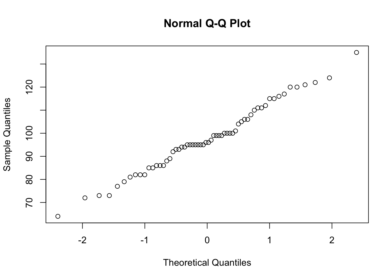

n    <- nrow(iq)
mean <- mean(iq$IQscore)
sd   <- sd(iq$IQscore)
se   <- sd / sqrt(n)
q_val<- qt(p = 0.025, df = n-1) 

mean + c(-1, 1)*se*abs(q_val)

[1]  93.99302 101.50698

Compare with t-test

t.test(iq$IQscore)$conf.int

[1]  93.99302 101.50698
attr(,"conf.level")
[1] 0.95

Install the libraries boot and simpleboot and load them (using the facilities under the tab Packages in R or RStudio, or using the commands in the R script.) Bootstrap the mean of the IQ scores, with R = 10000 resamples. Make a histogram and Normal quantile plot of the bootstrap distribution. Does the bootstrap distribution appear Normal? What is the bootstrap standard error? Give the bootstrap t 95% confidence interval.

Only need to do this once:

install.packages(c("boot", "simpleboot"))

library(boot)
library(simpleboot)

set.seed(12345)
bootresults <- one.boot(iq$IQscore, mean, R = 10000)

mean(bootresults$t); sd(bootresults$t)

[1] 97.73412

[1] 1.847751

qqnorm(bootresults$t)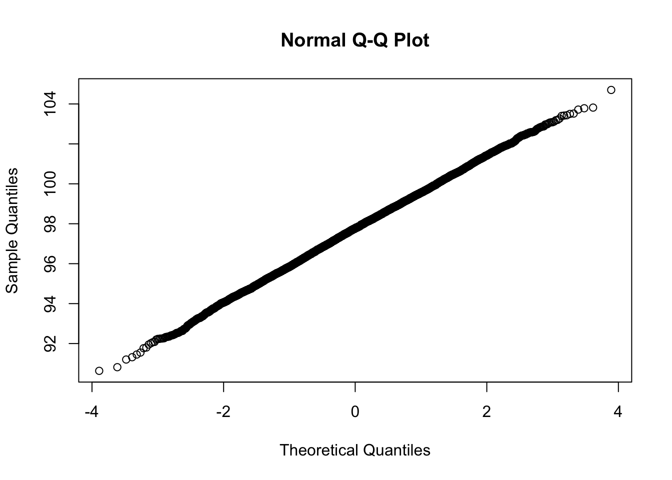

hist(bootresults$t)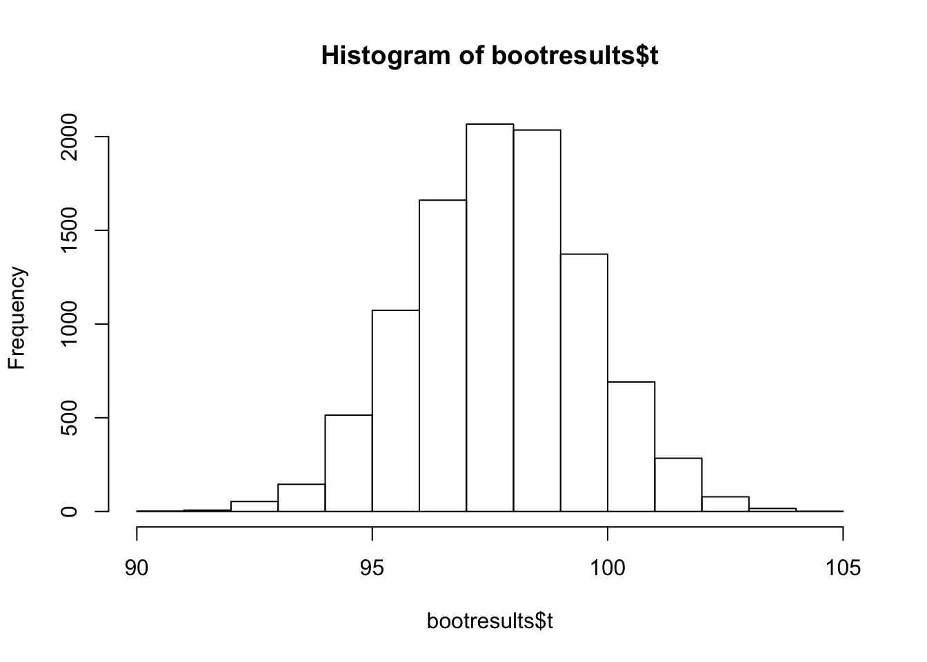

Looks nicely normally distributed.

Now for the 95% CI:

mean(bootresults$t) + c(-1,1)*qt(0.025, df = nrow(iq)-1, lower.tail = F)*sd(bootresults$t)/sqrt(nrow(iq))

[1] 97.25680 98.21145

Give the 95% confidence percentile, BCa, and basic intervals. How well do your five confidence intervals agree? Was bootstrapping needed to find a reasonable confidence interval, or was the formula-based confidence interval in (a) good enough?

boot.ci(bootresults)

Warning in boot.ci(bootresults): bootstrap variances needed for studentized
intervals

BOOTSTRAP CONFIDENCE INTERVAL CALCULATIONS
Based on 10000 bootstrap replicates

CALL : 
boot.ci(boot.out = bootresults)

Intervals : 
Level      Normal              Basic         
95%   ( 94.14, 101.39 )   ( 94.15, 101.38 )  

Level     Percentile            BCa          
95%   ( 94.12, 101.35 )   ( 94.08, 101.30 )  
Calculations and Intervals on Original Scale

The bootstrapping intervals agree, they are all a little narrower than the t-test based confidence interval, however the difference is small.

This is an (approximately) normally distributed vriable, so the t-test interval is accurate.

Ex. 16.65 A small-sample permutation test.

To illustrate the process, let’s perform a permutation test by hand for a small random subset of the DRP data (Example 16.11). Here are the data (different from those in the lecture): Treatment group 57 53 Control group 19 37 41 42 (a) Calculate the difference in means xtreatment − xcontrol between the two groups. This is the observed value of the statistic.

df <- data.frame(
  treat = c("treat", "treat", "control", "control", "control", "control"),
  x = c(57, 53, 19, 37, 41, 42)
)

diffx <- df %>% 
  group_by(treat) %>% 
  summarize(mean = mean(x)) %>%
  pull(mean) %>%
  diff()
diffx

[1] 20.25

Resample: randomly shuffle the 6 scores, where the two first scores will have the treatment (1), and the last 4 have control (0). What is the difference in group means for this resample?

set.seed(2)
df %>%
  mutate(treat = sample(treat)) %>% # shuffle treat
  group_by(treat) %>%
  summarize(mean = mean(x)) %>% # calculate mean by group
  pull(mean) %>%
  diff() # get difference

[1] 8.25

Repeat step (b) 1000 times to get 1000 resamples and 1000 values of the statistic. (Obviously you will not do this 1000 times by hand. Do it a few times by hand until you understand the procedure, then proceed with R.) Make a table of the distribution of these 1000 values. This is the permutation distribution for your resamples.

npermutations = 1000
set.seed(2)

diffs <- numeric(npermutations)

for (i in 1:npermutations) {
  diffs[i] <- df %>%
    mutate(treat = sample(treat)) %>% # shuffle treat
    group_by(treat) %>%
    summarize(mean = mean(x)) %>% # calculate mean by group
    pull(mean) %>%
    diff() # get difference
}

Look at the distribution of the differences

hist(diffs)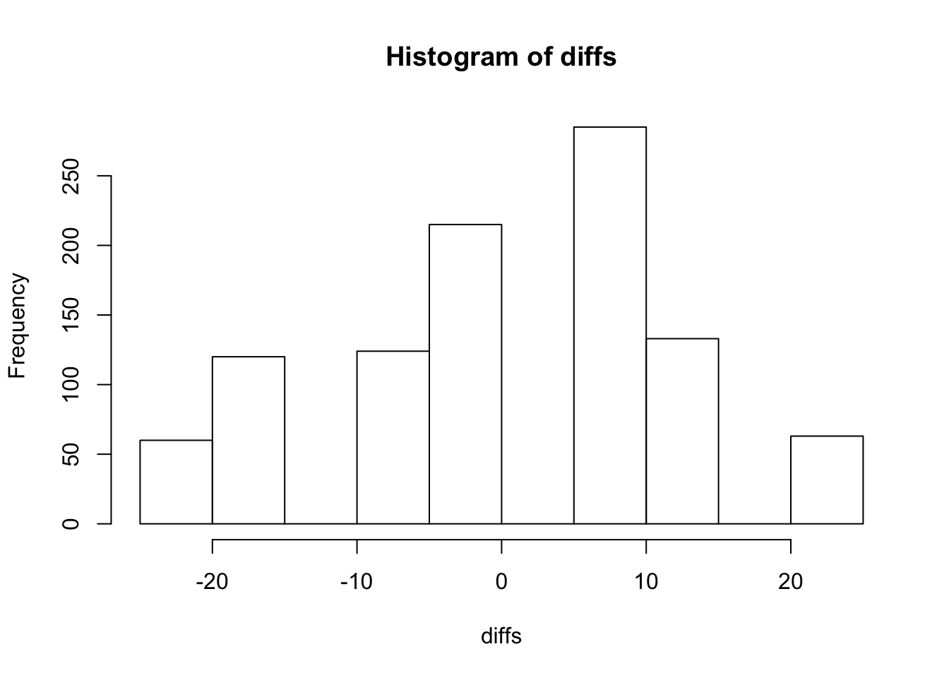

What proportion of the 1000 statistic values were equal to or greater than the original value in part (a)? You have just estimated the one-sided P-value for the original 6 observations.

mean(diffs >=diffx)

[1] 0.063

For this small data set, there are only 15 possible permutations of the data. As a result, we can calculate the exact P-value by counting the number of permutations with a statistic value greater than or equal to the original value and then dividing by 15. What is the exact P-value here? How close was your estimate?

Create all permutations by making a matrix with all the possible positions in the data where treatment can be located

treat_positions <- combn(6,2)
treat_positions

     [,1] [,2] [,3] [,4] [,5] [,6] [,7] [,8] [,9] [,10] [,11] [,12] [,13]
[1,]    1    1    1    1    1    2    2    2    2     3     3     3     4
[2,]    2    3    4    5    6    3    4    5    6     4     5     6     5
     [,14] [,15]
[1,]     4     5
[2,]     6     6

Calculate differences

possible_differences <- apply(treat_positions, 2, function(pos) {
  mean(df$x[pos]) - mean(df$x[-pos])
})
sort(possible_differences)

 [1] -20.25 -17.25 -16.50  -8.25  -5.25  -3.75  -3.00   0.00   5.25   8.25
[11]   8.25   9.00  11.25  12.00  20.25

mean(possible_differences >= diffx)

[1] 0.06666667

The exact p-value is pretty close

16.76 Comparing serum retinol levels.

The formal medical term for vitamin A in the blood is serum retinol. Serum retinol has various beneficial effects, such as protecting against fractures. Medical researchers working with children in Papua New Guinea asked whether recent infections reduce the level of serum retinol. They classified children as recently infected or not on the basis of other blood tests, then measured serum retinol. Of the 90 children in the sample, 55 had been recently infected. Dataset retinol.txt gives the serum retinol levels for both groups, in micromoles per liter. (a) The researchers are interested in the proportional reduction in serum retinol. Verify that the mean for infected children is 0.620 and that the mean for uninfected children is 0.778.

retinol <- read.table(fromParentDir("data/retinol.txt"), header = T)
str(retinol)

'data.frame':   90 obs. of  2 variables:
 $ retinol : num  0.59 1.08 0.88 0.62 0.46 0.39 1.44 1.04 0.67 0.86 ...
 $ infected: int  0 0 0 0 0 0 0 0 0 0 ...

retinol %>%
  group_by(infected) %>%
  summarize(mean(retinol))

# A tibble: 2 x 2
  infected `mean(retinol)`
     <int>           <dbl>
1        0           0.778
2        1           0.620

ratio <- retinol %>%
  group_by(infected) %>%
  summarize(mean = mean(retinol)) %>%
  pull(mean) %>%
  (function(x) (x/lag(x))[2])

There is no standard test for the null hypothesis that the ratio of the population means is 1. We can do a permutation test on the ratio of sample means. Carry out a one-sided test and report the P-value. Briefly describe the center and shape of the permutation distribution. Why do you expect the center to be close to 1?

First let’s calculate the number of possible permutations, to see if calculating all permutations is feasible

retinol %>% 
  group_by(infected) %>% # group by infected
  summarize(n = n())  # count number of infected

# A tibble: 2 x 2
  infected     n
     <int> <int>
1        0    35
2        1    55

choose(35+55, 55)

[1] 1.132459e+25

Getting all permutations is clearly infeasible, so let’s do 1000

nperm  = 1000
ratios = numeric(nperm)
set.seed(2)

for (i in 1:nperm) {
  ratios[i] <-
    retinol %>%
      mutate(shuff_intected = sample(infected)) %>%
      group_by(shuff_intected) %>%
      summarize(mean = mean(retinol)) %>%
      pull(mean) %>%
      (function(x) (x / lag(x))[2]) # divide each element by the previous, take second element (which is the fraction if x is 2 numbers)
}

hist(ratios)

Distributions looks pretty symmetric around 1, which is the null value for a ratio

qqnorm(ratios)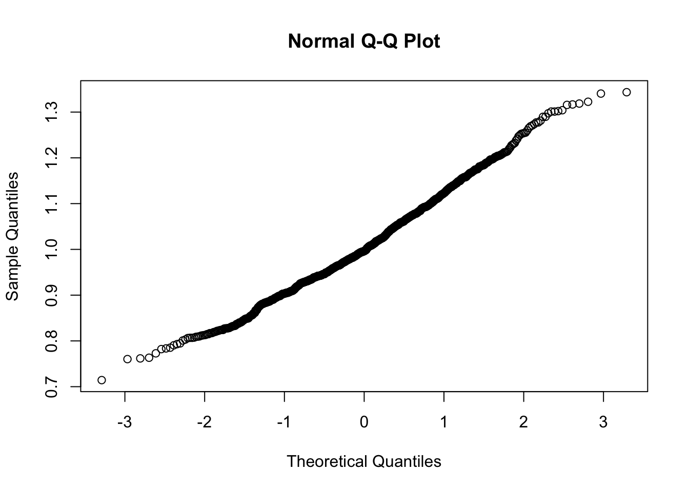

Pretty nice normal distribution

Now for the P-value

mean(ratios < ratio)

[1] 0.011

With plot for observed ratio

hist(ratios)
abline(v = ratio, lty = 2)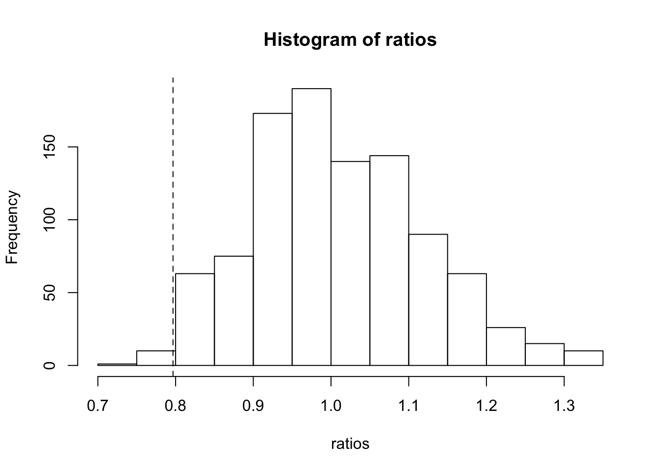

16.77 Methods of resampling.

In the previous exercise we did a permutation test for the hypothesis “no difference between infected and uninfected children” using the ratio of mean serum retinol levels to measure “difference.” We might also want a bootstrap confidence interval for the ratio of population means for infected and uninfected children. Describe carefully how resampling is done for the permutation test and for the bootstrap, paying attention to the difference between the two resampling methods.

Permution tests are used to simulate a distribution for the null-hypothesis. For this unpaired case it means shuffling the outcome (infected), which are expected to depend on the determinant (retinol). Under the null-hypothesis there is no relationship between the determinant and the outcome, so each possible configuration of outcomes is equially likely to occur. A number of random configurations is simulated, and the test statistic is calculated for each permution. This gives the distribution of the null-hypothesis. Based on this distribution, we can see how probable it is to find a value for the statistic or more extreme, which is the exact definition of a p-value. So permutations give p-values

Bootstrapping simulates drawing random samples from the population, but uses the actual observed distribution in the sample as a proxy for the population distribution (which is usually unknown if you’re doing research). Drawing re-samples from this sample distribution and calculating the test statistic for each re-sample gives an idea of the range of possible values of the statistic for a sample of the given size. This distrubution of the sample statistic can be used to approximate the confidence interval, which can (loosely) be defined as the range of values which a sample test statistic is (e.g. 95%) likelily to fall in between, when taking many samples.

Calcium intake and blood pressure. (Exercise from previous edition)

Does added calcium intake reduce the blood pressure of black men? In a randomized comparative double-blind trial, 10 men were given a calcium supplement for twelve weeks and 11 others received a placebo. Whether or not blood pressure dropped was recorded for each subject. Here are the data: Treatment Subjects Successes Proportion Calcium 10 6 0.60 Placebo 11 4 0.36 Total 21 10 0.48

calcium <- data.frame(
  treatment = rep(c(1, 0), c(10, 11)),
  success   = rep(c(1, 0, 1, 0), c(6, 4, 4, 7))
)
calcium

   treatment success
1          1       1
2          1       1
3          1       1
4          1       1
5          1       1
6          1       1
7          1       0
8          1       0
9          1       0
10         1       0
11         0       1
12         0       1
13         0       1
14         0       1
15         0       0
16         0       0
17         0       0
18         0       0
19         0       0
20         0       0
21         0       0

We want to use these sample data to test equality of the population proportions of successes. Carry out a permutation test. Describe the permutation distribution. The permutation test does not depend on a “nice” distribution shape. Give the P-value and report your conclusion.

The question here is to randomly divide 10 successes over 21 subjects.

The possible number of permutations:

choose(21, 10)

[1] 352716

This is doable.

We can get all the permutations by assigning 10 ‘rownumbers’ or positions for the successes in the 21 participants.

positions <- combn(21, 10)

positions[, 1:5]

      [,1] [,2] [,3] [,4] [,5]
 [1,]    1    1    1    1    1
 [2,]    2    2    2    2    2
 [3,]    3    3    3    3    3
 [4,]    4    4    4    4    4
 [5,]    5    5    5    5    5
 [6,]    6    6    6    6    6
 [7,]    7    7    7    7    7
 [8,]    8    8    8    8    8
 [9,]    9    9    9    9    9
[10,]   10   11   12   13   14

Let’s make sure that all treated participants are in the first 10 rows.

The the number of successes in the treatment group is the number of times a position of $\leq 10$ happens in the permuted positions. Let’s call this $n$, than the difference in ratios is $\frac{n}{10}-\frac{10-n}{11}$

diffs <- apply(positions, 2, function(position) {
  n = sum(position <= 10)
  (n/10) - ((10-n)/11)
})

Look at the distribution

hist(diffs)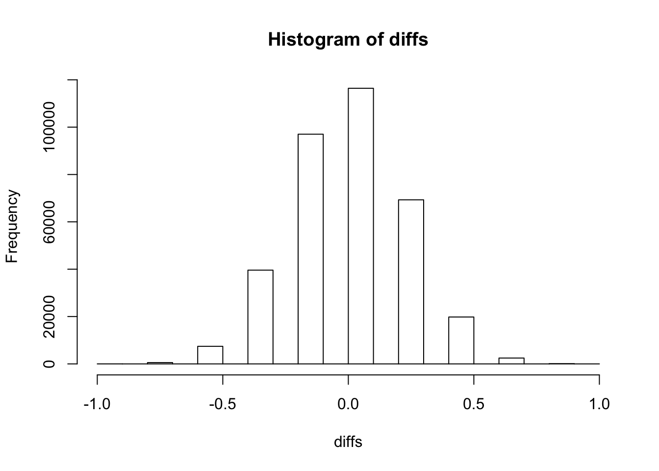

Compare with observed ratio to get a p-value

diffx <- 6/10 - 4 / 11

mean(diffx <= diffs)

[1] 0.2599428

Now check with pre-defined functions:

perm::permTS(calcium$success ~ calcium$treatment, alternative = "less", method = "exact.ce")


    Exact Permutation Test (complete enumeration)

data:  calcium$success by calcium$treatment
p-value = 0.2599
alternative hypothesis: true mean calcium$treatment=0 - mean calcium$treatment=1 is less than 0
sample estimates:
mean calcium$treatment=0 - mean calcium$treatment=1 
                                         -0.2363636

fisher.test(calcium$success, calcium$treatment, alternative = "greater")


    Fisher's Exact Test for Count Data

data:  calcium$success and calcium$treatment
p-value = 0.2599
alternative hypothesis: true odds ratio is greater than 1
95 percent confidence interval:
 0.436804      Inf
sample estimates:
odds ratio 
  2.502462

Our manual calculation coincides with Fisher’s test and permTS method

Internally, permTS does something similar as we did with the permutations It creates a ‘cm’ matrix with all possible combinations, the dimensions of this matrix is 352716x21. Check the code with:

View(permute:::permTS.default) which calls: View(permute:::twosample.exact.ce) which calls: View(permute:::chooseMatrix)

Now let’s do a more direct method, exploiting the fact that every combination of $n$ successes in the treatment group will yield the same results. Note: this only works when ‘success’ is a binary variable, it would not work in the more general case for continous outcomes.

n1 = 10
n2 = 11
ns = 10
diffx

[1] 0.2363636

perm_twogroup <- function(target, n1, n2, ns) {
  
  total_combinations <- choose(n1+n2, ns)
  combinations <- integer(ns+1)
  differences <- numeric(ns+1)
  
  for (n in 0:ns) {
    i = n+1
    
    difference = n / n1 - (ns-n) / n2
    ncombinations = choose(n1, n)*choose(n2, ns-n)
    
    differences[i] = difference
    combinations[i]= ncombinations
  }
  
  sum(combinations[differences>=target]) / total_combinations
  
}

perm_twogroup(diffx, n1, n2, ns)

[1] 0.2599428

Lets compare computation speed:

system.time(perm::permTS(calcium$success ~ calcium$treatment, alternative = "less", method = "exact.ce"))

   user  system elapsed 
  2.760   0.092   2.853

system.time(fisher.test(calcium$success, calcium$treatment, alternative = "greater"))

   user  system elapsed 
  0.001   0.000   0.001

system.time(perm_twogroup(diffx, n1, n2, ns))

   user  system elapsed 
      0       0       0

We can see that permTS is extremely slow, compared to fisher.test and the manual exact method.

Survival Exercises

1. Leukemia

We will have a closer look at the data from the lecture, on remission times for leukemia:

Read in the dataset leukaemia.txt (saved as a flat text file), changing your working directory first or adding the path name to the file name:

leuk<-read.table(fromParentDir("data/leukaemia.txt"), header = TRUE)

Fit five models (name them fit0 – fit4) with the following predictor variables: none (intercept only), GROUP, logWBCC, GROUP and logWBCC, GROUP*logWBCC. fit0<-coxph(Surv(TIME, STATUS)~1, data=leuk) etc.

require(survival)
fit0 <- coxph(Surv(TIME,  STATUS) ~ 1, data = leuk)
fit1 <- coxph(Surv(TIME,  STATUS) ~ GROUP, data = leuk)
fit2 <- coxph(Surv(TIME,  STATUS) ~ logWBCC, data = leuk)
fit3 <- coxph(Surv(TIME,  STATUS) ~ GROUP + logWBCC, data = leuk)
fit4 <- coxph(Surv(TIME,  STATUS) ~ GROUP * logWBCC, data = leuk)

Ask for the log-likelihood of the empty model: fit0$loglik Ask for the summaries of the 4 models fit1-fit4, and for their log-likelihoods.

fit0$loglik

[1] -93.18427

Let’s combine the summaries of the models by converting them to data.frames with broom, and bind them together with rbindlist

fits <- list(fit1, fit2, fit3, fit4)

summaries <- map(fits, broom::tidy) %>%
  data.table::rbindlist(idcol = "model")

summaries

   model                  term   estimate std.error  statistic
1:     1         GROUPtreatmnt -1.5721251 0.4123967 -3.8121670
2:     2               logWBCC  1.6464371 0.2979940  5.5250677
3:     3         GROUPtreatmnt -1.3860755 0.4247984 -3.2629020
4:     3               logWBCC  1.6908904 0.3358976  5.0339462
5:     4         GROUPtreatmnt -2.3749100 1.7054652 -1.3925291
6:     4               logWBCC  1.5548945 0.3986606  3.9002964
7:     4 GROUPtreatmnt:logWBCC  0.3175219 0.5257887  0.6038963
        p.value   conf.low  conf.high
1: 1.377538e-04 -2.3804079 -0.7638424
2: 3.293585e-08  1.0623795  2.2304946
3: 1.102776e-03 -2.2186651 -0.5534860
4: 4.804846e-07  1.0325432  2.3492376
5: 1.637622e-01 -5.7175604  0.9677404
6: 9.607498e-05  0.7735341  2.3362550
7: 5.459126e-01 -0.7130050  1.3480487

Interpret the coefficients of the models 1 through 4. What are you assuming with these models about the effect of group and logWBCC on the hazard of relapse?

require(data.table)
summaries[order(term)]

   model                  term   estimate std.error  statistic
1:     1         GROUPtreatmnt -1.5721251 0.4123967 -3.8121670
2:     3         GROUPtreatmnt -1.3860755 0.4247984 -3.2629020
3:     4         GROUPtreatmnt -2.3749100 1.7054652 -1.3925291
4:     4 GROUPtreatmnt:logWBCC  0.3175219 0.5257887  0.6038963
5:     2               logWBCC  1.6464371 0.2979940  5.5250677
6:     3               logWBCC  1.6908904 0.3358976  5.0339462
7:     4               logWBCC  1.5548945 0.3986606  3.9002964
        p.value   conf.low  conf.high
1: 1.377538e-04 -2.3804079 -0.7638424
2: 1.102776e-03 -2.2186651 -0.5534860
3: 1.637622e-01 -5.7175604  0.9677404
4: 5.459126e-01 -0.7130050  1.3480487
5: 3.293585e-08  1.0623795  2.2304946
6: 4.804846e-07  1.0325432  2.3492376
7: 9.607498e-05  0.7735341  2.3362550

In models 1 and 3 there is a significant group effect of GROUP (decreased hazard). In all models, logWBCC seems to have a significant effect. The interaction term of model 4 can be left out.

Estimates higher than 0 correspond with increased hazards. The exponent of this estimate gives the hazard ratio (leaving the rest the same)

Assumptions are proportional hazards, so the effects of group and logWBCC on the hazard do not depend on time (the hazard ratios are constant in time).

Calculate likelihood ratio test values and AIC’s (assume that the empty model, fit0, uses no degrees of freedom)

anova(fit0, fit1, fit2, fit3, fit4)

Analysis of Deviance Table
 Cox model: response is  Surv(TIME, STATUS)
 Model 1: ~ 1
 Model 2: ~ GROUP
 Model 3: ~ logWBCC
 Model 4: ~ GROUP + logWBCC
 Model 5: ~ GROUP * logWBCC
   loglik   Chisq Df P(>|Chi|)    
1 -93.184                         
2 -85.008 16.3517  1 5.261e-05 ***
3 -75.763 18.4899  0 < 2.2e-16 ***
4 -69.828 11.8708  1 0.0005702 ***
5 -69.648  0.3594  1 0.5488232    
---
Signif. codes:  0 '***' 0.001 '**' 0.01 '*' 0.05 '.' 0.1 ' ' 1

AIC(fit0, fit1, fit2, fit3, fit4)

Warning in is.na(coefficients(object)): is.na() applied to non-(list or
vector) of type 'NULL'

     df      AIC
fit0  0       NA
fit1  1 172.0168
fit2  1 153.5270
fit3  2 143.6562
fit4  3 145.2968

The lowest AIC is for fit3, both terms but no interaction. We already observed earlier on that the interaction term in model 4 was not significant, so it must be left out (AIC penalizes extra terms)

Also compare the models via the likelihood ratio test, with commands like anova(fit1, fit3, test=“Chisq”) Note that not all comparisons are possible.

anova(fit1, fit2, test = "Chisq")

Analysis of Deviance Table
 Cox model: response is  Surv(TIME, STATUS)
 Model 1: ~ GROUP
 Model 2: ~ logWBCC
   loglik Chisq Df P(>|Chi|)    
1 -85.008                       
2 -75.763 18.49  0 < 2.2e-16 ***
---
Signif. codes:  0 '***' 0.001 '**' 0.01 '*' 0.05 '.' 0.1 ' ' 1

The anova gives a result, but fit2 is not nested within fit1, so it’s meaningless.s

Decide which model is best. Interpret the coefficients of this best model.

We already saw that model 3 has the lowest AIC, so we will pick that one

summary(fit3)

Call:
coxph(formula = Surv(TIME, STATUS) ~ GROUP + logWBCC, data = leuk)

  n= 42, number of events= 30 

                 coef exp(coef) se(coef)      z Pr(>|z|)    
GROUPtreatmnt -1.3861    0.2501   0.4248 -3.263   0.0011 ** 
logWBCC        1.6909    5.4243   0.3359  5.034  4.8e-07 ***
---
Signif. codes:  0 '***' 0.001 '**' 0.01 '*' 0.05 '.' 0.1 ' ' 1

              exp(coef) exp(-coef) lower .95 upper .95
GROUPtreatmnt    0.2501     3.9991    0.1088    0.5749
logWBCC          5.4243     0.1844    2.8082   10.4776

Concordance= 0.852  (se = 0.062 )
Rsquare= 0.671   (max possible= 0.988 )
Likelihood ratio test= 46.71  on 2 df,   p=7.187e-11
Wald test            = 33.6  on 2 df,   p=5.061e-08
Score (logrank) test = 46.07  on 2 df,   p=9.921e-11

Treatment reduces the hazard, logWBCC increases the hazard

2. Nephrectomy

Researchers are interested in the influence of age nephrectomy on the survival of hypernephroma patients. Read the data below into R from the file nephrect.txt:

neph<-read.table(fromParentDir("data/nephrect.txt"), header = TRUE)
str(neph)

'data.frame':   36 obs. of  4 variables:
 $ survtime: int  9 6 21 15 8 17 12 104 9 56 ...
 $ status  : int  1 1 1 1 1 1 1 0 1 1 ...
 $ nephrect: int  0 0 0 0 0 0 0 1 1 1 ...
 $ age     : int  1 1 1 2 2 2 3 1 1 1 ...

Survival times of 36 hypernephroma patients classified according to age group and whether or not they have had a nephrectomy.

Make Kaplan-Meier plots for the three age groups, and test whether there is an effect of age on survival time (not taking nephrectomy into account) using the Log-rank test.

plot(survfit(Surv(survtime, status)~age, data = neph))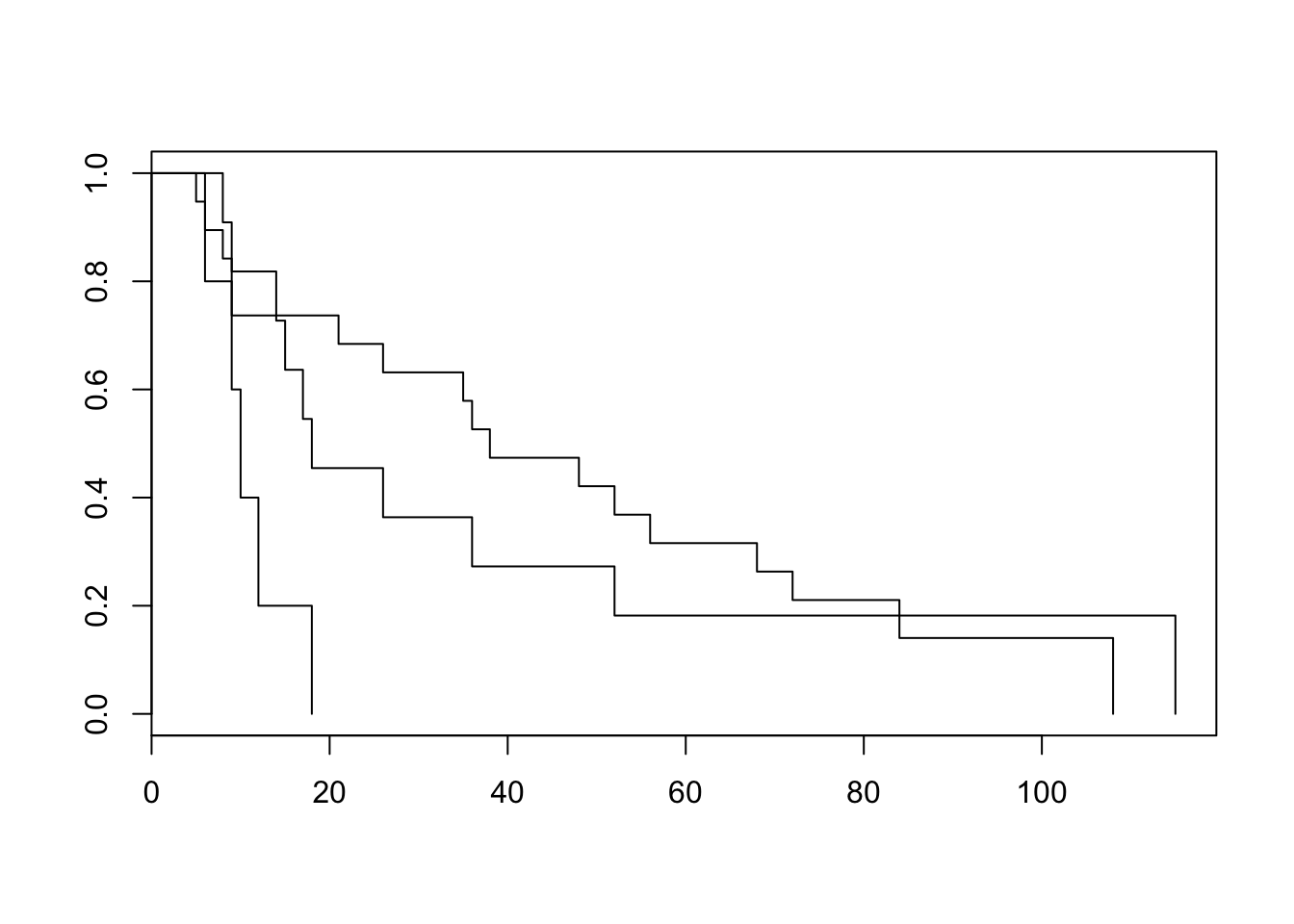

survdiff(Surv(survtime, status)~age, data = neph)

Call:
survdiff(formula = Surv(survtime, status) ~ age, data = neph)

       N Observed Expected (O-E)^2/E (O-E)^2/V
age=1 19       17    19.59    0.3424    1.0150
age=2 12       10    10.77    0.0554    0.0952
age=3  5        5     1.64    6.9042    8.2183

 Chisq= 8.3  on 2 degrees of freedom, p= 0.0161

According to the log-rank test, there is a significant difference in survival between age groups. (see documentation: the default for rho is 0, which corresponds to the log-rank test)

Test whether there is an effect of age on survival time (not taking nephrectomy into account) using the Likelihood Ratio test and the Wald test from a Cox Proportional Hazards regression model. (Define AGE as a categorical variable.) Compare this result to the log-rank test.

fit1 <- coxph(Surv(survtime, status) ~ factor(age), data = neph)
summary(fit1)

Call:
coxph(formula = Surv(survtime, status) ~ factor(age), data = neph)

  n= 36, number of events= 32 

               coef exp(coef) se(coef)     z Pr(>|z|)   
factor(age)2 0.1010    1.1063   0.4204 0.240  0.81004   
factor(age)3 1.5144    4.5467   0.5807 2.608  0.00911 **
---
Signif. codes:  0 '***' 0.001 '**' 0.01 '*' 0.05 '.' 0.1 ' ' 1

             exp(coef) exp(-coef) lower .95 upper .95
factor(age)2     1.106     0.9039    0.4853     2.522
factor(age)3     4.547     0.2199    1.4569    14.189

Concordance= 0.602  (se = 0.054 )
Rsquare= 0.148   (max possible= 0.993 )
Likelihood ratio test= 5.79  on 2 df,   p=0.05542
Wald test            = 7.09  on 2 df,   p=0.02881
Score (logrank) test = 8.4  on 2 df,   p=0.01498

The log-rank gives the lowest p-value. Likelihood ratio test is not significant

From the Cox PH output, give the hazard ratio of age class 2 vs 1 and 3 vs 1. Give the 95% confidence intervals for these hazard ratios. Interpret the results.

broom::tidy(fit1) %>%
  mutate_at(.vars = c("estimate", "conf.low", "conf.high"), exp)

          term estimate std.error statistic     p.value  conf.low
1 factor(age)2 1.106331 0.4203911 0.2403689 0.810044275 0.4853415
2 factor(age)3 4.546690 0.5806640 2.6080477 0.009106028 1.4569116
  conf.high
1  2.521869
2 14.189183

Hazard ratios are the estimates (exponentiated as required). For the 2 vs 1 hazard ratio, the confidence interval includes the null value of 1, which coincides with the p.value of > 0.05

Now take only nephrectomy as the explanatory variable. Make Kaplan-Meier plots for the two groups, test for a difference in nephrectomy status using the log-rank test.

plot(survfit(Surv(survtime, status)~nephrect, data = neph))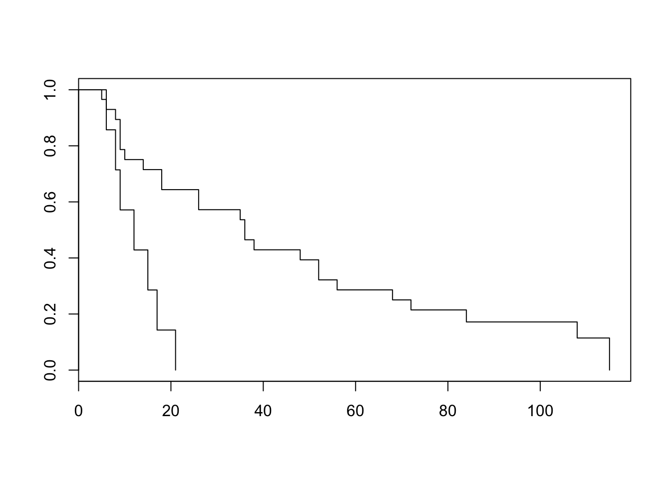

survdiff(Surv(survtime, status)~nephrect, data = neph)

Call:
survdiff(formula = Surv(survtime, status) ~ nephrect, data = neph)

            N Observed Expected (O-E)^2/E (O-E)^2/V
nephrect=0  7        7     2.46     8.408      10.5
nephrect=1 29       25    29.54     0.699      10.5

 Chisq= 10.5  on 1 degrees of freedom, p= 0.00122

Test whether there is an effect of nephrectomy using the likelihood ratio and Wald tests in a Cox PH model. Compare this result to the log-rank test. Give the hazard ratio of no nephrectomy vs nephrectomy. Calculate a 95% confidence interval for this hazard ratio.

fit2 <- coxph(Surv(survtime, status)~nephrect, data = neph)
summary(fit2)

Call:
coxph(formula = Surv(survtime, status) ~ nephrect, data = neph)

  n= 36, number of events= 32 

            coef exp(coef) se(coef)      z Pr(>|z|)   
nephrect -1.4941    0.2245   0.5070 -2.947  0.00321 **
---
Signif. codes:  0 '***' 0.001 '**' 0.01 '*' 0.05 '.' 0.1 ' ' 1

         exp(coef) exp(-coef) lower .95 upper .95
nephrect    0.2245      4.455    0.0831    0.6063

Concordance= 0.598  (se = 0.037 )
Rsquare= 0.19   (max possible= 0.993 )
Likelihood ratio test= 7.56  on 1 df,   p=0.005955
Wald test            = 8.69  on 1 df,   p=0.003208
Score (logrank) test = 10.31  on 1 df,   p=0.00132

exp(coef(fit2))

 nephrect 
0.2244505

exp(confint((fit2)))

              2.5 %    97.5 %
nephrect 0.08309507 0.6062696

Nefrectomy seems to have a lower hazard of dying

Test for a difference in nephrectomy status using a Cox PH model again, but now for each of the three original age classes separately (hint: make 3 new data frames with selections of age groups). Does the effect of nephrecto¬my appear to be the same in each age class? (Optional: how would you test this, using Cox PH?)

Let’s do this with dplyr function group_by

fits <- neph %>%
  group_by(age) %>%
  do(fit = coxph(Surv(survtime, status)~nephrect, data = .))

broom::tidy(fits, fit)

# A tibble: 3 x 8
# Groups:   age [3]
    age term     estimate std.error statistic p.value conf.low conf.high
  <int> <chr>       <dbl>     <dbl>     <dbl>   <dbl>    <dbl>     <dbl>
1     1 nephrect   -2.00      0.827    -2.42   0.0156    -3.62   -0.379 
2     2 nephrect   -1.71      0.922    -1.86   0.0629    -3.52    0.0923
3     3 nephrect    0.370     1.19      0.311  0.755     -1.96    2.70

The estimate for nephrectomy is different in the different age groups, however, the confidence intervals all overlap.

We can test this by using age as an interaction

fit2 <- coxph(Surv(survtime, status)~nephrect*factor(age), data = neph)
summary(fit2)

Call:
coxph(formula = Surv(survtime, status) ~ nephrect * factor(age), 
    data = neph)

  n= 36, number of events= 32 

                           coef exp(coef)  se(coef)      z Pr(>|z|)   
nephrect              -1.996683  0.135785  0.729653 -2.736  0.00621 **
factor(age)2          -0.032209  0.968304  0.836657 -0.038  0.96929   
factor(age)3           0.002361  1.002364  1.179871  0.002  0.99840   
nephrect:factor(age)2  0.002939  1.002944  0.971967  0.003  0.99759   
nephrect:factor(age)3  2.140991  8.507868  1.342752  1.594  0.11083   
---
Signif. codes:  0 '***' 0.001 '**' 0.01 '*' 0.05 '.' 0.1 ' ' 1

                      exp(coef) exp(-coef) lower .95 upper .95
nephrect                 0.1358     7.3646   0.03249    0.5675
factor(age)2             0.9683     1.0327   0.18787    4.9909
factor(age)3             1.0024     0.9976   0.09925   10.1236
nephrect:factor(age)2    1.0029     0.9971   0.14926    6.7393
nephrect:factor(age)3    8.5079     0.1175   0.61216  118.2424

Concordance= 0.653  (se = 0.057 )
Rsquare= 0.354   (max possible= 0.993 )
Likelihood ratio test= 15.75  on 5 df,   p=0.007586
Wald test            = 14.94  on 5 df,   p=0.01061
Score (logrank) test = 19.98  on 5 df,   p=0.00126

Interaction term is indeed not significant

Check the Cox PH assumption for AGE by building a model with NEPHRECT as explanatory variable and AGE as stratum variable. Get a log-minus-log plot and check whether the resulting log cumulative hazard functions are approximately parallel.

fit3 <- coxph(Surv(survtime, status)~nephrect + strata(factor(age)), data = neph)
summary(fit3)

Call:
coxph(formula = Surv(survtime, status) ~ nephrect + strata(factor(age)), 
    data = neph)

  n= 36, number of events= 32 

            coef exp(coef) se(coef)      z Pr(>|z|)  
nephrect -1.3077    0.2705   0.5399 -2.422   0.0154 *
---
Signif. codes:  0 '***' 0.001 '**' 0.01 '*' 0.05 '.' 0.1 ' ' 1

         exp(coef) exp(-coef) lower .95 upper .95
nephrect    0.2705      3.698   0.09387    0.7792

Concordance= 0.607  (se = 0.055 )
Rsquare= 0.14   (max possible= 0.962 )
Likelihood ratio test= 5.42  on 1 df,   p=0.0199
Wald test            = 5.87  on 1 df,   p=0.01543
Score (logrank) test = 6.57  on 1 df,   p=0.01035

The fast way:

plot(survfit(fit3), col = c("red", "blue", "black"), fun = "cloglog")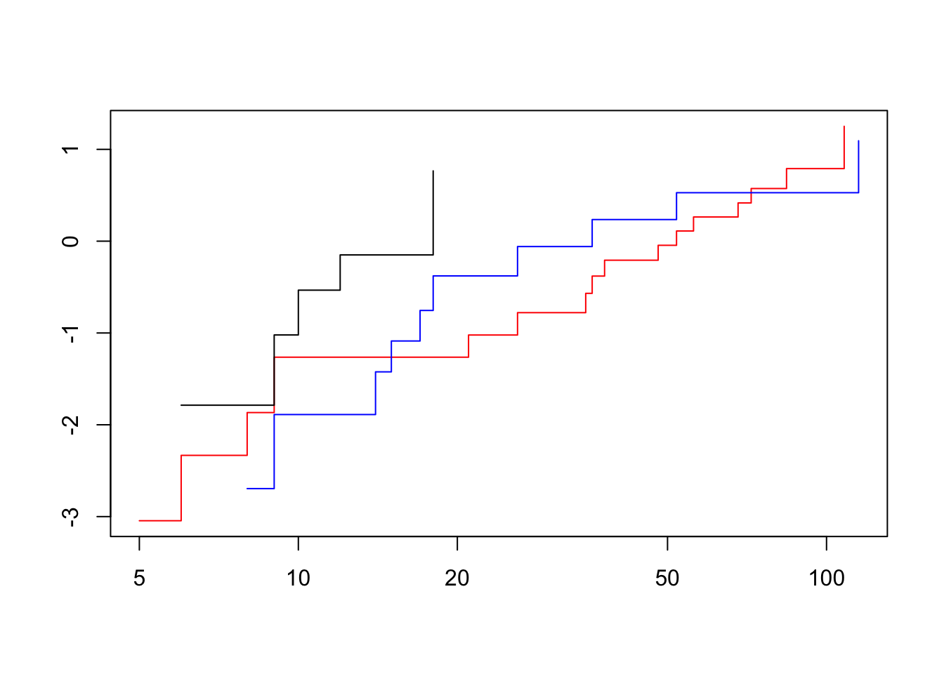

The lines cross, so this vialates our assumption of proportional hazards

3. Myeloma

Read the data file myeloma.dat (a comma-separated file with headers at the top) into R and attach it:

myel<-read.table(fromParentDir("data/myeloma.dat"), header = TRUE)
str(myel)

'data.frame':   48 obs. of  10 variables:
 $ patient: int  1 2 3 4 5 6 7 8 9 10 ...
 $ time   : int  13 52 6 40 10 7 66 10 10 14 ...
 $ status : int  1 0 1 1 1 0 1 0 1 1 ...
 $ age    : int  66 66 53 69 65 57 52 60 70 70 ...
 $ sex    : int  1 1 0 1 1 0 1 1 1 1 ...
 $ bun    : int  25 13 15 10 20 12 21 41 37 40 ...
 $ ca     : int  10 11 13 10 10 8 10 9 12 11 ...
 $ hb     : num  14.6 12 11.4 10.2 13.2 9.9 12.8 14 7.5 10.6 ...
 $ pc     : int  18 100 33 30 66 45 11 70 47 27 ...
 $ bj     : int  1 0 1 1 0 0 1 1 0 0 ...

The dataset contains the following variables on 48 patients diagnosed with multiple myeloma: Variable Description survtime survival time from diagnosis multiple myeloma (months) status censoring status (0=censored, 1=death from multiple myeloma) age age (years) sex sex (1=male, 2=female) bun blood urea nitrogen ca serum calcium hb haemoglobin pc percentage plasma cells in bone marrow bj Bence-Jones protein in urine

The object of the research is to determine the best fitting Cox proportional hazards model to explain death from multiple myeloma.

First, get some descriptive statistics on the data. Then get a sense of the individual variables’ effect on survival, by fitting a Cox PH model on each of the explanatory variables separately.

summary(myel)

    patient           time           status          age       
 Min.   : 1.00   Min.   : 1.00   Min.   :0.00   Min.   :50.00  
 1st Qu.:12.75   1st Qu.: 6.75   1st Qu.:0.75   1st Qu.:58.75  
 Median :24.50   Median :14.50   Median :1.00   Median :62.50  
 Mean   :24.50   Mean   :23.38   Mean   :0.75   Mean   :62.90  
 3rd Qu.:36.25   3rd Qu.:37.00   3rd Qu.:1.00   3rd Qu.:68.25  
 Max.   :48.00   Max.   :91.00   Max.   :1.00   Max.   :77.00  
      sex              bun               ca               hb       
 Min.   :0.0000   Min.   :  6.00   Min.   : 8.000   Min.   : 4.90  
 1st Qu.:0.0000   1st Qu.: 13.75   1st Qu.: 9.000   1st Qu.: 8.65  
 Median :1.0000   Median : 21.00   Median :10.000   Median :10.20  
 Mean   :0.6042   Mean   : 33.92   Mean   : 9.938   Mean   :10.25  
 3rd Qu.:1.0000   3rd Qu.: 39.25   3rd Qu.:10.000   3rd Qu.:12.57  
 Max.   :1.0000   Max.   :172.00   Max.   :15.000   Max.   :14.60  
       pc               bj        
 Min.   :  3.00   Min.   :0.0000  
 1st Qu.: 21.25   1st Qu.:0.0000  
 Median : 33.00   Median :0.0000  
 Mean   : 42.94   Mean   :0.3125  
 3rd Qu.: 63.00   3rd Qu.:1.0000  
 Max.   :100.00   Max.   :1.0000

Let’s model all variables separately (except for patient, time and status)

vars <- setdiff(colnames(myel), c("patient", "time", "status"))

fits <- map(vars, .f = function(var) {
  fit = coxph(Surv(time, status)~get(var), data = myel)
})
names(fits) <- vars

fits_summary <- map_dfr(fits, broom::tidy, .id = "var")
fits_summary

  var     term     estimate   std.error  statistic     p.value
1 age get(var)  0.010370389 0.027974456  0.3707092 0.710854121
2 sex get(var) -0.064606144 0.354630810 -0.1821786 0.855442567
3 bun get(var)  0.020151980 0.005726557  3.5190396 0.000433112
4  ca get(var) -0.088886279 0.132472799 -0.6709776 0.502234810
5  hb get(var) -0.134673527 0.059294189 -2.2712770 0.023130216
6  pc get(var)  0.001587994 0.005680465  0.2795535 0.779820101
7  bj get(var) -0.553957353 0.387880839 -1.4281637 0.153244733
      conf.low   conf.high
1 -0.044458538  0.06519932
2 -0.759669760  0.63045747
3  0.008928135  0.03137582
4 -0.348528193  0.17075564
5 -0.250888002 -0.01845905
6 -0.009545514  0.01272150
7 -1.314189828  0.20627512

Now, fit an empty model (no explanatory variables), and use the forward method (use the add1() function, the option test=”Chisq” for a likelihood ratio test, and the scope option to indicate which variables may be included) to build a final model.

fit0 <- coxph(Surv(time, status)~1, data = myel)

add1(fit0, scope = vars, test = "Chisq")

Warning in is.na(fit$coefficients): is.na() applied to non-(list or vector)
of type 'NULL'

Single term additions

Model:
Surv(time, status) ~ 1
       Df    AIC    LRT Pr(>Chi)   
<none>    214.68                   
age     1 216.54 0.1378 0.710431   
sex     1 216.65 0.0330 0.855821   
bun     1 207.32 9.3624 0.002215 **
ca      1 216.20 0.4746 0.490884   
hb      1 211.66 5.0169 0.025101 * 
pc      1 216.60 0.0773 0.780977   
bj      1 214.51 2.1680 0.140913   
---
Signif. codes:  0 '***' 0.001 '**' 0.01 '*' 0.05 '.' 0.1 ' ' 1

fit1 <- coxph(Surv(time, status)~bun, data = myel)
add1(fit1, scope = vars, test = "Chisq")

Single term additions

Model:
Surv(time, status) ~ bun
       Df    AIC    LRT Pr(>Chi)  
<none>    207.32                  
age     1 209.32 0.0000  0.99531  
sex     1 209.30 0.0144  0.90438  
bun     0 207.32 0.0000           
ca      1 209.28 0.0398  0.84194  
hb      1 204.70 4.6171  0.03165 *
pc      1 209.04 0.2805  0.59635  
bj      1 204.99 4.3274  0.03750 *
---
Signif. codes:  0 '***' 0.001 '**' 0.01 '*' 0.05 '.' 0.1 ' ' 1

fit2 <- coxph(Surv(time, status)~bun+hb, data = myel)
add1(fit2, scope = vars, test = "Chisq")

Single term additions

Model:
Surv(time, status) ~ bun + hb
       Df    AIC     LRT Pr(>Chi)  
<none>    204.70                   
age     1 206.45 0.24630   0.6197  
sex     1 206.31 0.39250   0.5310  
bun     0 204.70 0.00000           
ca      1 206.70 0.00067   0.9794  
hb      0 204.70 0.00000           
pc      1 206.47 0.22516   0.6351  
bj      1 203.90 2.79772   0.0944 .
---
Signif. codes:  0 '***' 0.001 '**' 0.01 '*' 0.05 '.' 0.1 ' ' 1

No more significant improvements

The re¬searchers also wish to know whether the effects of the risk factors might be modified by the age or sex of a patient, so, in the final model, test for possible interactions with these two. Note: to fit the interaction term you will also have to fit the main effect (age or sex).

fit3 <- coxph(Surv(time, status)~(bun+hb)*(age + sex), data = myel)
summary(fit3)

Call:
coxph(formula = Surv(time, status) ~ (bun + hb) * (age + sex), 
    data = myel)

  n= 48, number of events= 36 

              coef  exp(coef)   se(coef)      z Pr(>|z|)
bun     -0.0005735  0.9994266  0.0402039 -0.014    0.989
hb      -0.3425636  0.7099480  0.6870670 -0.499    0.618
age     -0.0640206  0.9379857  0.1125184 -0.569    0.569
sex      0.2781463  1.3206795  1.4752258  0.189    0.850
bun:age  0.0003291  1.0003291  0.0006804  0.484    0.629
bun:sex  0.0031629  1.0031679  0.0120207  0.263    0.792
hb:age   0.0030344  1.0030391  0.0104302  0.291    0.771
hb:sex  -0.0151251  0.9849887  0.1445146 -0.105    0.917

        exp(coef) exp(-coef) lower .95 upper .95
bun        0.9994     1.0006    0.9237     1.081
hb         0.7099     1.4086    0.1847     2.729
age        0.9380     1.0661    0.7524     1.169
sex        1.3207     0.7572    0.0733    23.796
bun:age    1.0003     0.9997    0.9990     1.002
bun:sex    1.0032     0.9968    0.9798     1.027
hb:age     1.0030     0.9970    0.9827     1.024
hb:sex     0.9850     1.0152    0.7420     1.308

Concordance= 0.675  (se = 0.06 )
Rsquare= 0.275   (max possible= 0.989 )
Likelihood ratio test= 15.46  on 8 df,   p=0.05081
Wald test            = 17.62  on 8 df,   p=0.02428
Score (logrank) test = 21.28  on 8 df,   p=0.006433

There seems to be no significant interaction

drop1(fit3)

Single term deletions

Model:
Surv(time, status) ~ (bun + hb) * (age + sex)
        Df    AIC
<none>     215.22
bun:age  1 213.45
bun:sex  1 213.29
hb:age   1 213.31
hb:sex   1 213.23

Dropping the interactions improves the model, so final model is model 2

Interpret the coefficients from your final model (direction and size of the hazard ratios).

summary(fit2)

Call:
coxph(formula = Surv(time, status) ~ bun + hb, data = myel)

  n= 48, number of events= 36 

         coef exp(coef)  se(coef)      z Pr(>|z|)    
bun  0.020043  1.020245  0.005816  3.446 0.000569 ***
hb  -0.134952  0.873758  0.061956 -2.178 0.029391 *  
---
Signif. codes:  0 '***' 0.001 '**' 0.01 '*' 0.05 '.' 0.1 ' ' 1

    exp(coef) exp(-coef) lower .95 upper .95
bun    1.0202     0.9802    1.0087    1.0319
hb     0.8738     1.1445    0.7738    0.9866

Concordance= 0.67  (se = 0.06 )
Rsquare= 0.253   (max possible= 0.989 )
Likelihood ratio test= 13.98  on 2 df,   p=0.0009213
Wald test            = 16.11  on 2 df,   p=0.0003173
Score (logrank) test = 19.54  on 2 df,   p=5.712e-05

bun increases the hazard of dying (see exp(coef) for hazard ratio) hb decreases the hazard of dying (see exp(coef) for hazard ratio)

4. Nephrectomy SPSS

This exercise is a repeat of exercise 2, but in SPSS. Read the data from exercise 2 into SPSS (File, Read Text Data) from the file NEPHRECT.TXT.

This one was skipped

5. Myeloma SPSS

This exercise is a repeat of exercise 3, but in SPSS. Open the data file MYELOMA.POR. Use Utilities, Variables… to study the meaning of the variables in the data file.

This one was skipped

Longitudinal data

Exercise 1:

We will start by reproducing the results of this morning’s lecture concerning the milk protein data: Start R, load the library nlme and access the data set Milk:

library(nlme)
data(Milk)
summary(Milk)

    protein           Time             Cow                  Diet    
 Min.   :2.450   Min.   : 1.000   B02    :  19   barley       :425  
 1st Qu.:3.200   1st Qu.: 5.000   B17    :  19   barley+lupins:459  
 Median :3.410   Median : 9.000   B24    :  19   lupins       :453  
 Mean   :3.422   Mean   : 9.185   B09    :  19                      
 3rd Qu.:3.630   3rd Qu.:13.000   B11    :  19                      
 Max.   :4.590   Max.   :19.000   B05    :  19                      
                                  (Other):1223

In our analysis we will at first confine ourselves to time points 1 and 2:

Milk12<-Milk[Milk$Time<3,]
summary(Milk12)

    protein           Time            Cow                 Diet   
 Min.   :2.690   Min.   :1.000   B04    :  2   barley       :49  
 1st Qu.:3.380   1st Qu.:1.000   B14    :  2   barley+lupins:54  
 Median :3.660   Median :1.000   B03    :  2   lupins       :54  
 Mean   :3.684   Mean   :1.497   B02    :  2                     
 3rd Qu.:3.980   3rd Qu.:2.000   B16    :  2                     
 Max.   :4.590   Max.   :2.000   B17    :  2                     
                                 (Other):145

To calculate the mean for protein type the command

If we want to calculate the mean for the different weeks we can make use of the tapply function

Or use dplyr

tapply(Milk12$protein,Milk12$Time,mean)

       1        2 
3.834051 3.532692

Milk12 %>%
  group_by(Time) %>%
  summarize(mean(protein))

# A tibble: 2 x 2
   Time `mean(protein)`
  <dbl>           <dbl>
1  1.00            3.83
2  2.00            3.53

To avoid that we have to include the name of the dataset every time we name a variable, we will attach the data set to the search list:

Let’s not do this

So now R will also look in the dataset Milk12 to look for objects that you use in your commands. So after attaching the dataset it will suffice to write

Make a “spaghetti plot” of the protein data for weeks 1 and 2:

with(Milk12,
     interaction.plot(x.factor=Time,trace.factor=Cow,response=protein))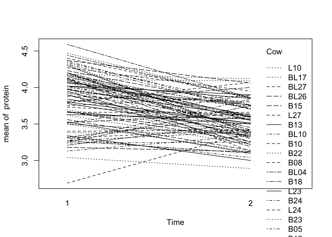

We will now do a pooled T test and a paired T test on the data. Since cow “B20” has a missing protein value at time 2, we will delete this cow from the data set for now.

Milk12complete<-Milk12 %>% filter(Cow!="B20")
str(Milk12complete)

'data.frame':   156 obs. of  4 variables:
 $ protein: num  3.63 3.57 3.24 3.25 3.98 3.6 3.66 3.5 4.34 3.76 ...
 $ Time   : num  1 2 1 2 1 2 1 2 1 2 ...
 $ Cow    : Ord.factor w/ 79 levels "B04"<"B14"<"B03"<..: 25 25 4 4 3 3 1 1 16 16 ...
 $ Diet   : Factor w/ 3 levels "barley","barley+lupins",..: 1 1 1 1 1 1 1 1 1 1 ...
 - attr(*, "formula")=Class 'formula'  language protein ~ Time | Cow
  .. ..- attr(*, ".Environment")=<environment: R_GlobalEnv> 
 - attr(*, "units")=List of 2
  ..$ x: chr "(weeks)"
  ..$ y: chr "(%)"
 - attr(*, "outer")=Class 'formula'  language ~Diet
  .. ..- attr(*, ".Environment")=<environment: R_GlobalEnv> 
 - attr(*, "FUN")=function (x)  
 - attr(*, "order.groups")= logi TRUE

(Note that dataset Milk12complete is added to the search list before Milk12, so R will look in Milk12Bcomplete first. Variables in Milk12 are “masked”.)

t.test(protein~Time,var.equal=T, data = Milk12complete)


    Two Sample t-test

data:  protein by Time
t = 5.3923, df = 154, p-value = 2.568e-07
alternative hypothesis: true difference in means is not equal to 0
95 percent confidence interval:
 0.1910686 0.4120083
sample estimates:
mean in group 1 mean in group 2 
       3.834231        3.532692

t.test(protein~Time,paired=T, data = Milk12complete)


    Paired t-test

data:  protein by Time
t = 7.1354, df = 77, p-value = 4.601e-10
alternative hypothesis: true difference in means is not equal to 0
95 percent confidence interval:
 0.2173894 0.3856875
sample estimates:
mean of the differences 
              0.3015385

Note that both T tests give highly significant results but the p value from the paired T test is much smaller: 2.610-7 vs. 4.610-10.

We can do equivalent analyses using ANOVA (Oneway and split-plot, respectively). This enables us to compare sums-of-squares of the ANOVA tables:

summary(aov(protein~Time, data = Milk12complete))

             Df Sum Sq Mean Sq F value   Pr(>F)    
Time          1  3.546   3.546   29.08 2.57e-07 ***
Residuals   154 18.781   0.122                     
---
Signif. codes:  0 '***' 0.001 '**' 0.01 '*' 0.05 '.' 0.1 ' ' 1

summary(aov(protein~Time+Error(Cow), data = Milk12complete))


Error: Cow
          Df Sum Sq Mean Sq F value Pr(>F)
Residuals 77  13.42  0.1743               

Error: Within
          Df Sum Sq Mean Sq F value  Pr(>F)    
Time       1  3.546   3.546   50.91 4.6e-10 ***
Residuals 77  5.363   0.070                    
---
Signif. codes:  0 '***' 0.001 '**' 0.01 '*' 0.05 '.' 0.1 ' ' 1

Note that SS(Residuals) of the One-way ANOVA is the same as the sum of the two SS residuals in the Split-plot ANOVA. It is split into a “between Cow” and “Within” part.

To get an idea about the distribution of protein for week 1 and week 2, we can produce a scatter plot and a boxplot by executing:

plot(protein~Time, data = Milk12complete)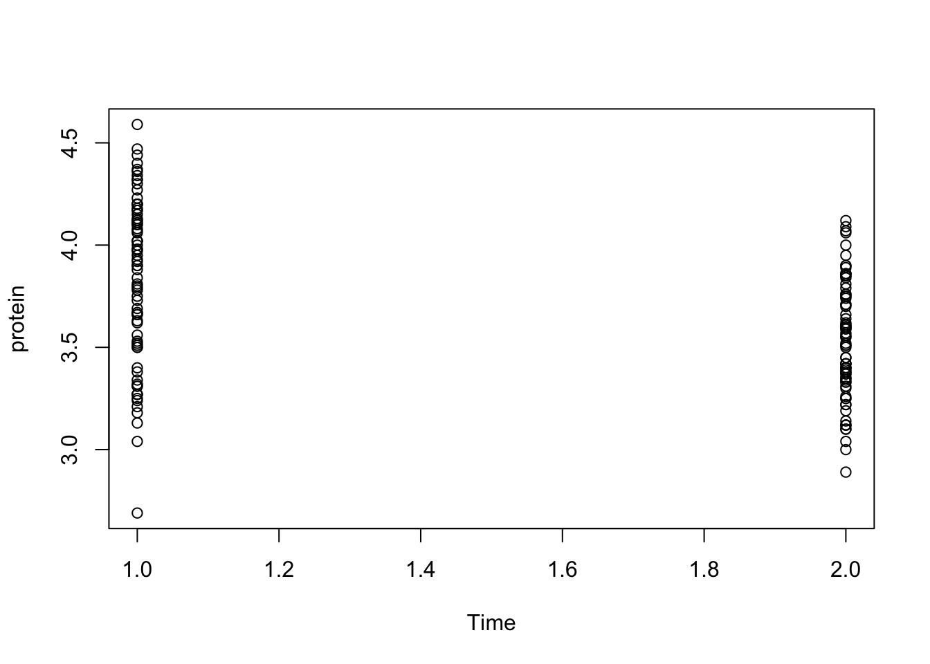

boxplot(protein~Time, data = Milk12complete)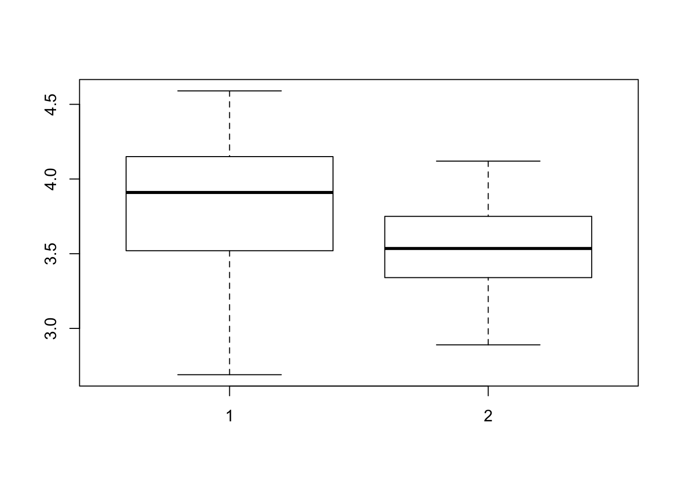

If we want to calculate the mean protein per diet for every week and make a plot of them, we just have to execute the commands

# tapply(protein,list(Diet,Time),mean)

Milk12complete %>%
  group_by(Diet, Time) %>%
  summarize(mean(protein))

# A tibble: 6 x 3
# Groups:   Diet [?]
  Diet           Time `mean(protein)`
  <fct>         <dbl>           <dbl>
1 barley         1.00            3.89
2 barley         2.00            3.64
3 barley+lupins  1.00            3.86
4 barley+lupins  2.00            3.54
5 lupins         1.00            3.76
6 lupins         2.00            3.43

with(Milk12complete,
     interaction.plot(x.factor=Time,trace.factor=Diet,response=protein))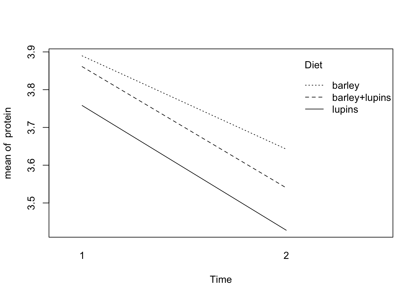

# tapply(protein,list(Diet,Time),var)
Milk12complete %>%
  group_by(Time, Diet) %>%
  summarize(mean = mean(protein), var = var(protein))

# A tibble: 6 x 4
# Groups:   Time [?]
   Time Diet           mean    var
  <dbl> <fct>         <dbl>  <dbl>
1  1.00 barley         3.89 0.149 
2  1.00 barley+lupins  3.86 0.143 
3  1.00 lupins         3.76 0.199 
4  2.00 barley         3.64 0.0567
5  2.00 barley+lupins  3.54 0.0774
6  2.00 lupins         3.43 0.0890

shows that the variances per diet in week 1 are much larger than in week 2.

To produce histograms for the protein observations per diet per week

library(lattice)        #Contains the function histogram
histogram(~protein | Time*Diet, data = Milk12complete)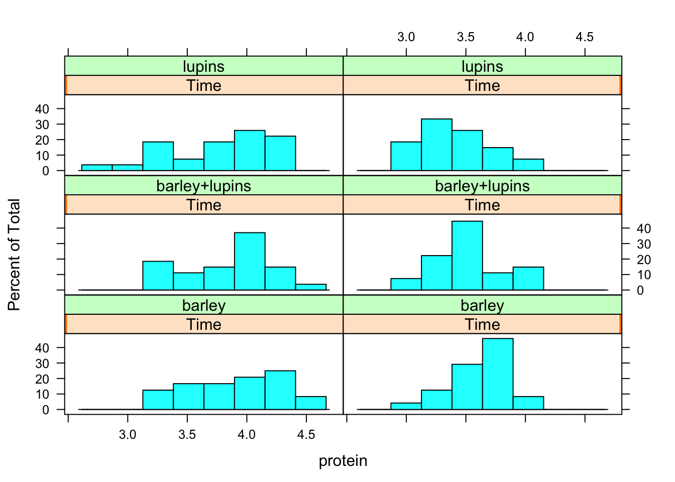

GGplot equivalent:

Milk12complete %>%
  ggplot(aes(x = protein)) +
  geom_histogram() +
  facet_grid(Diet~Time, scales = "fixed")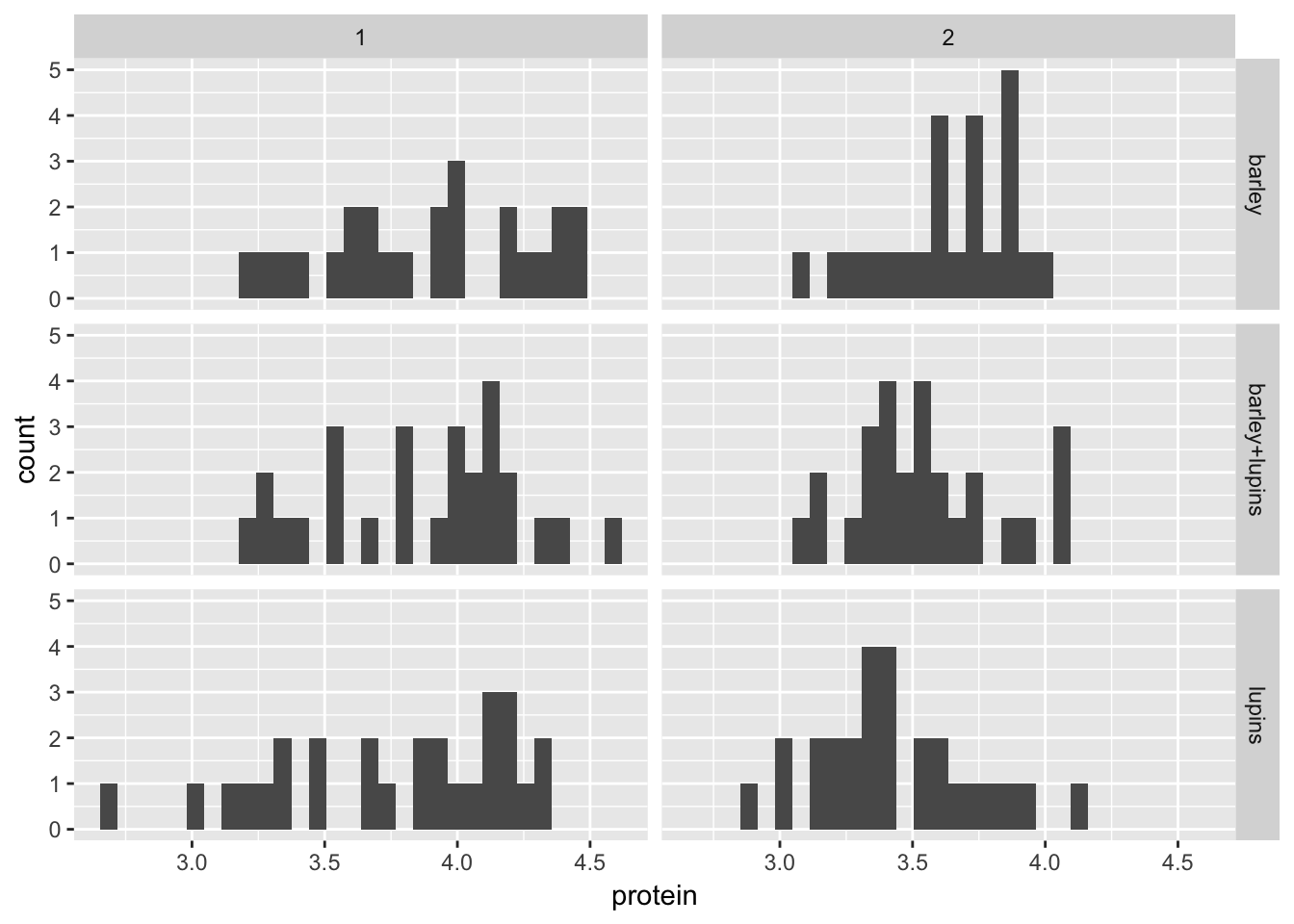

Comparing ggplot with lattice, we can see that the binwidth is pretty important

Let’s do 10 bins

Milk12complete %>%
  ggplot(aes(x = protein)) +
  geom_histogram(bins = 10) +
  facet_grid(Diet~Time, scales = "fixed")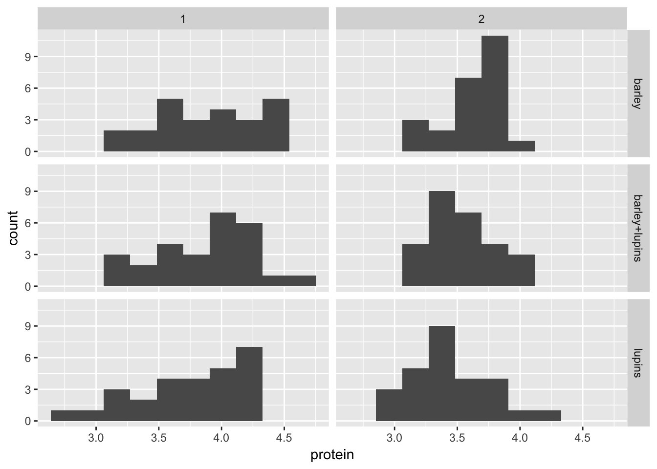

You can see that the histograms are more spread out in week 1.

We will now extend the analysis to the first 3 weeks, complete cases.

# Milk123complete<-Milk[Milk$Time<4 & Milk$Cow!="B20",]
Milk123complete<- Milk %>%
  filter(Time<4 & Cow!="B20")
with(Milk123complete,
     interaction.plot(x.factor=Time,trace.factor=Diet,response=protein))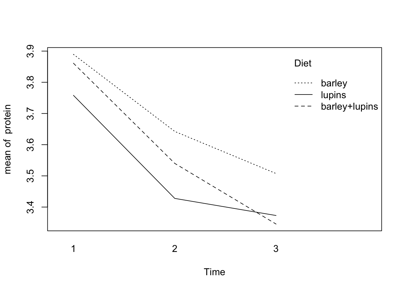

Let’s first investigate the protein profiles per cow graphically. (Normally we would have to tell R that our observations are grouped. We could accomplish this by creating a new groupedData set, where cow is our grouping variable: d.gr <-groupedData(protein~Time|Cow, data=Milk123complete) Here, the internal dataset Milk was already grouped.)

For a plot of all cows together (like the spaghetti interaction.plot), run

plot(Milk123complete,outer=~1,aspect=1,key=F)

This command does not work for me, probably because some package makes some alteration to the plot function (it’s not lattice).

Let’s do it ‘by hand’

Milk123complete %>%
  ggplot(aes(x = Time, y = protein, col = Cow)) + 
  geom_line() + 
  theme(legend.position = "none")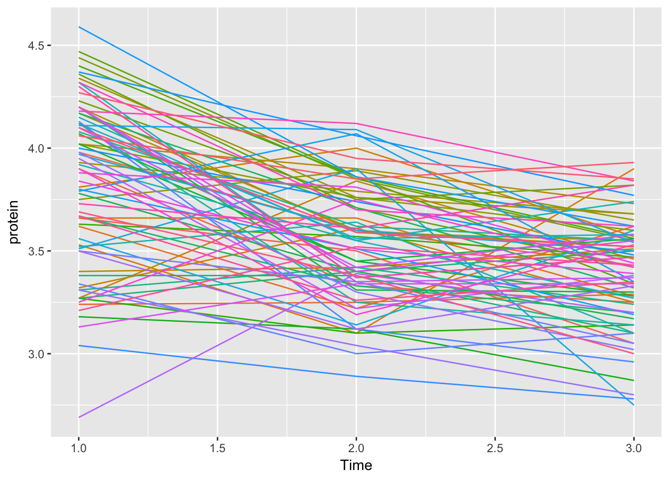

(key=F suppresses the elaborate non-informative legend.) For the same plot, but now per diet group, run

plot(Milk123complete,outer=~Diet,layout=c(3,1),aspect=1,key=F)

Again this doesn’t work, but GGplot2 can do the job

Milk123complete %>%
  ggplot(aes(x = Time, y = protein, col = Cow)) + 
  geom_line() + 
  facet_grid(~Diet, scales = "fixed") + 
  theme(legend.position = "none")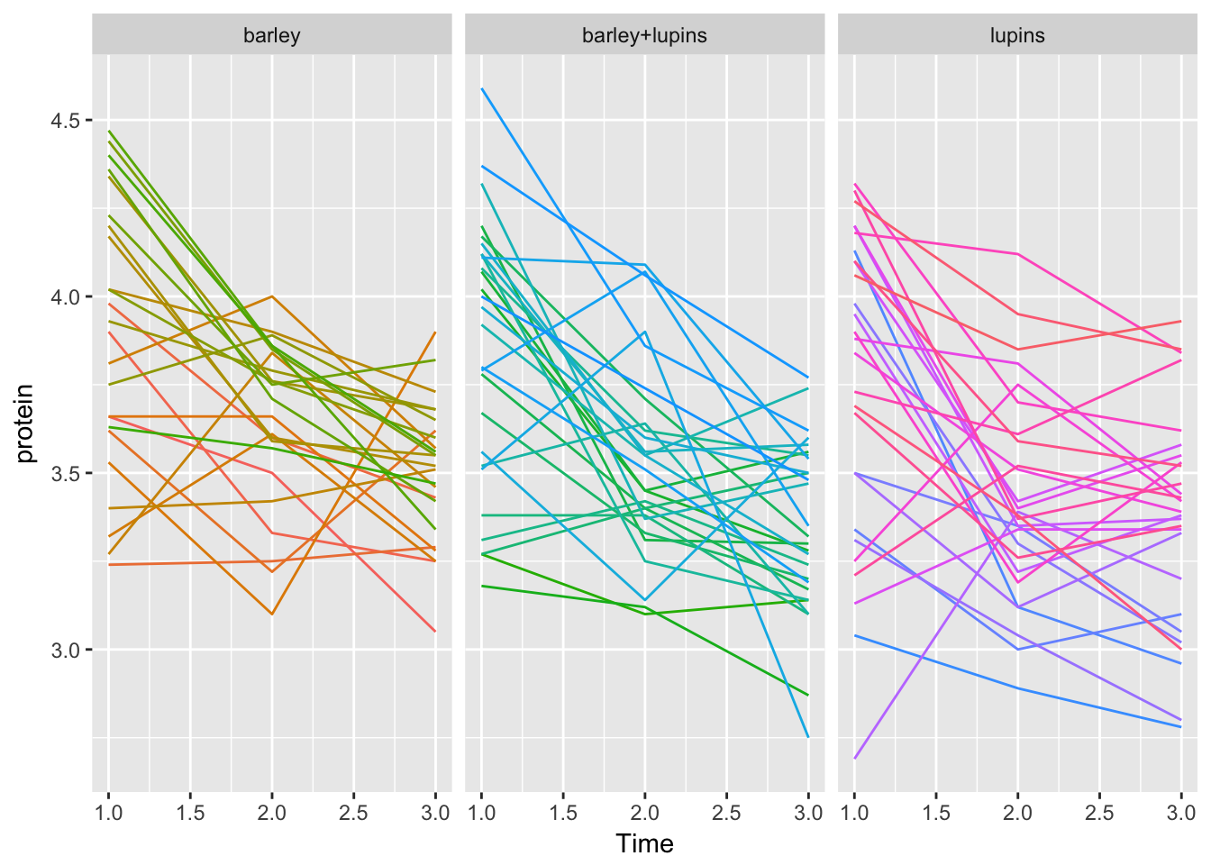

In the next part we will produce the slope as summary measure for each cow over the first three weeks of observation. To calculate our summary measure (the slope) for every cow we fit a linear model per cow. The “lmList” function (which works on groupedData objects) will calculate the slopes and intercepts for a linear regression model with protein as dependent variable and Time as predictor. This is done for each cow separately. The results are stored in the object “fits”. Typing “fits” then displays these results:

fits<-lmList(protein~Time|Cow, data=Milk123complete)
fits

Call:
  Model: protein ~ Time | Cow 
   Data: Milk123complete 

Coefficients:
     (Intercept)          Time
B04     4.013333 -3.050000e-01
B14     4.143333 -3.250000e-01
B03     4.220000 -2.750000e-01
B02     3.210000  2.500000e-02
B16     3.486667 -3.925231e-16
B17     3.913333 -1.900000e-01
B21     3.140000  1.850000e-01
B25     3.463333 -3.500000e-02
B15     4.033333 -1.200000e-01
B24     3.333333  9.500000e-02
B09     3.333333  5.500000e-02
B13     4.173333 -1.450000e-01
B07     4.413333 -3.250000e-01
B11     4.430000 -3.250000e-01
B05     4.586667 -3.300000e-01
B23     4.050000 -1.250000e-01
B10     3.863333 -5.000000e-02
B12     4.213333 -2.100000e-01
B18     4.836667 -4.450000e-01
B19     4.343333 -2.050000e-01
B06     4.770000 -4.700000e-01
B22     5.020000 -5.650000e-01
B08     4.780000 -4.200000e-01
B01     3.716667 -8.000000e-02
BL18    3.300000 -6.500000e-02
BL16    3.366667 -1.550000e-01
BL15    4.323333 -3.700000e-01
BL05    4.203333 -2.550000e-01
BL11    4.503333 -4.500000e-01
BL24    4.060000 -3.050000e-01
BL03    4.583333 -4.250000e-01
BL08    3.870000 -2.350000e-01
BL19    3.160000  1.150000e-01
BL01    3.566667 -1.400000e-01
BL21    3.393333 -3.500000e-02
BL14    4.280000 -2.650000e-01
BL22    4.483333 -4.900000e-01
BL13    3.840000 -2.100000e-01
BL23    3.916667 -9.000000e-02
BL06    4.570000 -4.250000e-01
BL12    4.293333 -2.700000e-01
BL09    4.536667 -4.400000e-01
BL20    4.160000 -2.350000e-01
BL07    3.393333  2.000000e-02
BL10    4.146667 -3.800000e-01
BL17    4.483333 -2.850000e-01
BL27    4.176667 -2.200000e-01
BL02    4.110000 -3.050000e-01
BL04    4.993333 -4.850000e-01
BL26    4.666667 -3.000000e-01
BL25    4.260000 -2.600000e-01
L07     3.163333 -1.300000e-01
L16     4.573333 -5.850000e-01
L14     3.386667 -1.200000e-01
L15     3.750000 -2.250000e-01
L09     4.393333 -4.800000e-01
L03     3.560000 -2.550000e-01
L19     3.486667 -8.500000e-02
L21     2.583333  2.550000e-01
L25     4.086667 -2.850000e-01
L02     4.470000 -4.150000e-01
L20     4.220000 -2.600000e-01
L04     3.060000  1.050000e-01
L11     4.366667 -3.250000e-01
L24     4.150000 -2.200000e-01
L08     4.030000 -2.250000e-01
L13     3.303333  8.500000e-02
L18     3.910000 -1.850000e-01
L06     4.580000 -3.500000e-01
L10     4.386667 -1.700000e-01
L05     3.630000  4.500000e-02
L22     4.543333 -4.150000e-01
L17     3.166667  1.100000e-01
L26     3.746667 -1.600000e-01
L12     4.316667 -2.900000e-01
L01     4.046667 -3.450000e-01
L27     4.443333 -2.100000e-01
L23     4.076667 -6.500000e-02

Degrees of freedom: 234 total; 78 residual
Residual standard error: 0.2315855

Note that there is a substantial amount of variation in intercepts and slopes. (It might be worthwhile to try to take this into account. We’ll do that tomorrow.)

And here is a “little trick” to extract the slopes for every cow (using the fact that the slope is the second coefficient of the first part of the output):

slopes<-rep(0,78)
for(i in 1:78)slopes[i]<-fits[[i]][1]$coefficients[2]

(Note: the first of these two commands “initializes” slopes to be a vector consisting of 78 zeroes. The second command replaces these zeroes with the actual slopes.)

Here’s another way of doing this with the function map from purrr

slopes2 <- fits %>% 
  map("coefficients") %>% # grab coefficients
  map_dbl(2)              # grab 2nd element

cbind(slopes, slopes2)[1:10,]

           slopes       slopes2
B04 -3.050000e-01 -3.050000e-01
B14 -3.250000e-01 -3.250000e-01
B03 -2.750000e-01 -2.750000e-01
B02  2.500000e-02  2.500000e-02
B16 -3.925231e-16 -3.925231e-16
B17 -1.900000e-01 -1.900000e-01
B21  1.850000e-01  1.850000e-01
B25 -3.500000e-02 -3.500000e-02
B15 -1.200000e-01 -1.200000e-01
B24  9.500000e-02  9.500000e-02

This gives the same result, but depending on personal preference, the syntax may be a easier to read

From the output we see that the first 24 estimated lines belong to the cows on the Barley diet, the next 27 lines for the Mixed diet cows and the last 27 for cows on the Lupins diet. To link them to the diets, make a new variable:

DIET<-factor(c(rep(0,24),rep(1,27),rep(2,27)),labels=c("B","BL","L"))

To obtain the overall ANOVA table and estimates for the mean slope per diet:

summary(aov(slopes~DIET))

            Df Sum Sq Mean Sq F value Pr(>F)
DIET         2 0.0767 0.03837   1.163  0.318
Residuals   75 2.4733 0.03298

summary(lm(slopes~-1+DIET))


Call:
lm(formula = slopes ~ -1 + DIET)

Residuals:
     Min       1Q   Median       3Q      Max 
-0.39241 -0.13357 -0.01309  0.11018  0.44759 

Coefficients:
       Estimate Std. Error t value Pr(>|t|)    
DIETB  -0.19104    0.03707  -5.154 2.00e-06 ***
DIETBL -0.25778    0.03495  -7.376 1.82e-10 ***
DIETL  -0.19259    0.03495  -5.511 4.82e-07 ***
---
Signif. codes:  0 '***' 0.001 '**' 0.01 '*' 0.05 '.' 0.1 ' ' 1

Residual standard error: 0.1816 on 75 degrees of freedom
Multiple R-squared:  0.5975,    Adjusted R-squared:  0.5814 
F-statistic: 37.11 on 3 and 75 DF,  p-value: 8.21e-15

If we do not use the slope as a summary measure, but take the observations themselves, we can again calculate means and variances by:

# tapply(protein, list(Diet,Time), mean)
# tapply(protein, list(Diet,Time), var)

Milk123complete %>%
  group_by(Time, Diet) %>%
  summarize(mean(protein), var(protein))

# A tibble: 9 x 4
# Groups:   Time [?]
   Time Diet          `mean(protein)` `var(protein)`
  <dbl> <fct>                   <dbl>          <dbl>
1  1.00 barley                   3.89         0.149 
2  1.00 barley+lupins            3.86         0.143 
3  1.00 lupins                   3.76         0.199 
4  2.00 barley                   3.64         0.0567
5  2.00 barley+lupins            3.54         0.0774
6  2.00 lupins                   3.43         0.0890
7  3.00 barley                   3.51         0.0391
8  3.00 barley+lupins            3.35         0.0624
9  3.00 lupins                   3.37         0.0955

We can test the main effects and their interaction using ANOVA (either Twoway or split-plot) with diet and time as factors:

summary(aov(protein~Diet*factor(Time), data = Milk123complete))

                   Df Sum Sq Mean Sq F value   Pr(>F)    
Diet                2  0.987   0.494   4.840  0.00875 ** 
factor(Time)        2  7.582   3.791  37.166 1.13e-14 ***
Diet:factor(Time)   4  0.225   0.056   0.552  0.69762    
Residuals         225 22.950   0.102                     
---
Signif. codes:  0 '***' 0.001 '**' 0.01 '*' 0.05 '.' 0.1 ' ' 1

summary(aov(protein~Diet*factor(Time)+Error(Cow), data = Milk123complete))


Error: Cow
          Df Sum Sq Mean Sq F value Pr(>F)  
Diet       2  0.987  0.4937   2.592 0.0816 .
Residuals 75 14.284  0.1905                 
---
Signif. codes:  0 '***' 0.001 '**' 0.01 '*' 0.05 '.' 0.1 ' ' 1

Error: Within
                   Df Sum Sq Mean Sq F value Pr(>F)    
factor(Time)        2  7.582   3.791  65.620 <2e-16 ***
Diet:factor(Time)   4  0.225   0.056   0.975  0.423    
Residuals         150  8.666   0.058                   
---
Signif. codes:  0 '***' 0.001 '**' 0.01 '*' 0.05 '.' 0.1 ' ' 1

And finally, to fit a linear mixed effects (LME) model with random intercept:

lme.fit<-lme(fixed=protein~ Diet*factor(Time), random=~1|Cow, data = Milk123complete)
anova(lme.fit)

                  numDF denDF   F-value p-value
(Intercept)           1   150 15839.928  <.0001
Diet                  2    75     2.592  0.0816
factor(Time)          2   150    65.620  <.0001
Diet:factor(Time)     4   150     0.975  0.4231

summary(lme.fit)

Linear mixed-effects model fit by REML
 Data: Milk123complete 
       AIC      BIC    logLik
  137.7676 175.3447 -57.88379

Random effects:
 Formula: ~1 | Cow
        (Intercept)  Residual
StdDev:   0.2103056 0.2403568

Fixed effects: protein ~ Diet * factor(Time) 
                                    Value  Std.Error  DF  t-value p-value
(Intercept)                      3.889583 0.06519198 150 59.66353  0.0000
Dietbarley+lupins               -0.028472 0.08959780  75 -0.31778  0.7515
Dietlupins                      -0.131435 0.08959780  75 -1.46695  0.1466
factor(Time)2                   -0.247083 0.06938505 150 -3.56105  0.0005
factor(Time)3                   -0.382083 0.06938505 150 -5.50671  0.0000
Dietbarley+lupins:factor(Time)2 -0.074028 0.09536062 150 -0.77629  0.4388
Dietlupins:factor(Time)2        -0.083287 0.09536062 150 -0.87339  0.3838
Dietbarley+lupins:factor(Time)3 -0.133472 0.09536062 150 -1.39966  0.1637
Dietlupins:factor(Time)3        -0.003102 0.09536062 150 -0.03253  0.9741
 Correlation: 
                                (Intr) Dtbrl+ Dtlpns fc(T)2 fc(T)3 D+:(T)2
Dietbarley+lupins               -0.728                                    
Dietlupins                      -0.728  0.529                             
factor(Time)2                   -0.532  0.387  0.387                      
factor(Time)3                   -0.532  0.387  0.387  0.500               
Dietbarley+lupins:factor(Time)2  0.387 -0.532 -0.282 -0.728 -0.364        
Dietlupins:factor(Time)2         0.387 -0.282 -0.532 -0.728 -0.364  0.529 
Dietbarley+lupins:factor(Time)3  0.387 -0.532 -0.282 -0.364 -0.728  0.500 
Dietlupins:factor(Time)3         0.387 -0.282 -0.532 -0.364 -0.728  0.265 
                                D:(T)2 D+:(T)3
Dietbarley+lupins                             
Dietlupins                                    
factor(Time)2                                 
factor(Time)3                                 
Dietbarley+lupins:factor(Time)2               
Dietlupins:factor(Time)2                      
Dietbarley+lupins:factor(Time)3  0.265        
Dietlupins:factor(Time)3         0.500  0.529 

Standardized Within-Group Residuals:
         Min           Q1          Med           Q3          Max 
-3.208399150 -0.530625159 -0.006804944  0.523269323  2.125327364 

Number of Observations: 234
Number of Groups: 78

From the estimates of the coefficient values, how can you calculate predictions for the protein values for each of the 3 diets, at each of the 3 time points? (Answer: add the appropriate coefficients to get: Time 1 Time 2 Time 3 Barley 3.889583 3.642500 3.507500 Barley + lupins 3.861111 3.540000 3.345556 Lupins 3.758148 3.427778 3.372963

For each time-point add intercept the interaction terms. e.g. for lupins, time 3

3.889583+(-.131435)+(-.382083)+(-.003102)

[1] 3.372963

To get them all in 2 (or 3 for pretty printing) lines of codes:

grid <- expand.grid(Diet = unique(Milk123complete$Diet), 
                    Time = unique(factor(Milk123complete$Time)))
grid$predictions <- predict(lme.fit, newdata = grid, level = 0)
xtabs(predictions~Diet+Time, data = grid)

               Time
Diet                   1        2        3
  barley        3.889583 3.642500 3.507500
  barley+lupins 3.861111 3.540000 3.345556
  lupins        3.758148 3.427778 3.372963

This works as follows:

expand.grid creates a data.frame of all possible combinations of the supplied vectors
predict will predict the protein based on the supplied model.
- level = 0 is needed, which means ignore grouping (‘Cow’), otherwise the function will throw an error and ask for the grouping variable (so you will have to provide a Cow name)
xtabs is just to print it nicely

Clean up, by detaching the appropriate milk data files from the search list.

We didn’t attach, so no cleaning up required

Exercise 2:

The file Twisk1.dat contains longitudinal data concerning cholesterol measurements on several occasions. Furthermore, information about baseline values as well as time varying covariates is collected. id : patient number chol: serum cholesterol fitness: max oxygen uptake (baseline) skinfold: sum of four skin folds (time varying) smoke: does the patient smoke? (time varying, 0=no, 1=yes) gender: gender (factor, 1=male, 2=female) time: time in weeks (1-6)

Read the data into an R object and summarize it by

Twisk1<-read.table(fromParentDir("data/Twisk1.dat"),header=T)
summary(Twisk1)

       id             chol        fitness         skinfold     
 Min.   :  1.0   Min.   :2.4   Min.   :1.460   Min.   : 1.570  
 1st Qu.: 81.0   1st Qu.:3.9   1st Qu.:1.830   1st Qu.: 2.530  
 Median :270.0   Median :4.4   Median :1.970   Median : 3.370  
 Mean   :228.8   Mean   :4.5   Mean   :1.976   Mean   : 3.743  
 3rd Qu.:367.0   3rd Qu.:5.0   3rd Qu.:2.140   3rd Qu.: 4.688  
 Max.   :471.0   Max.   :7.5   Max.   :2.530   Max.   :12.210  
     smoke            gender           time    
 Min.   :0.0000   Min.   :1.000   Min.   :1.0  
 1st Qu.:0.0000   1st Qu.:1.000   1st Qu.:2.0  
 Median :0.0000   Median :2.000   Median :3.5  
 Mean   :0.1746   Mean   :1.531   Mean   :3.5  
 3rd Qu.:0.0000   3rd Qu.:2.000   3rd Qu.:5.0  
 Max.   :1.0000   Max.   :2.000   Max.   :6.0

Turn the variables id into a factor by Twisk1$id<-factor(Twisk1$id) Do the same for smoke and gender, and attach Twisk1 to the search list.

Let’s do this with dplyr for convenience

Twisk1 %<>% 
  mutate_at(vars(id, smoke, gender), factor)

Give mean and variance of the continuous variables chol, fitness and skinfold for all time points combined.

Here’s how to do this with dplyr

Twisk1 %>%
  summarize_at(vars(chol, fitness, skinfold), funs(mean, var))

  chol_mean fitness_mean skinfold_mean  chol_var fitness_var skinfold_var
1  4.499773     1.975714      3.743424 0.6607037  0.04790329     2.341117

Here with dplyr, purrr and data.table (admittably a little cumbersome, but this works for 30 variables and 20 functions too)

Twisk1 %>%
  select(chol, fitness, skinfold) %>%
  map(function(x) data.frame(mean(x), var(x))) %>%
  data.table::rbindlist(idcol = "variable")

   variable  mean.x.     var.x.
1:     chol 4.499773 0.66070369
2:  fitness 1.975714 0.04790329
3: skinfold 3.743424 2.34111743

Calculate these means and variances for every time point separately.

Just 1 extra line compared to a)

Twisk1 %>%
  group_by(time) %>%
  summarize_at(vars(chol, fitness, skinfold), funs(mean, var))

# A tibble: 6 x 7
   time chol_mean fitness_mean skinfold_mean chol_var fitness_var
  <int>     <dbl>        <dbl>         <dbl>    <dbl>       <dbl>
1     1      4.43         1.98          3.26    0.454      0.0482
2     2      4.32         1.98          3.36    0.443      0.0482
3     3      4.27         1.98          3.57    0.499      0.0482
4     4      4.17         1.98          3.76    0.493      0.0482
5     5      4.68         1.98          4.35    0.619      0.0482
6     6      5.13         1.98          4.16    0.856      0.0482
# ... with 1 more variable: skinfold_var <dbl>

How many females are there in the sample? Use tapply with function table to obtain frequency tables at each time point..

table(Twisk1$time, Twisk1$gender)

Use Twisk.gr<-groupedData(chol~time|id,data=Twisk1) to create a grouped dataset. Investigate graphically the individual profiles, also try to produce a graph where the profiles are shown by gender (outer=~gender). Warning: on some computers this may take some time, if you get bored press the escape key (several times).

Twisk1 %>%
  ggplot(aes(x = time, y = chol, col = id)) + 
  geom_line() + 
  theme(legend.position = "none")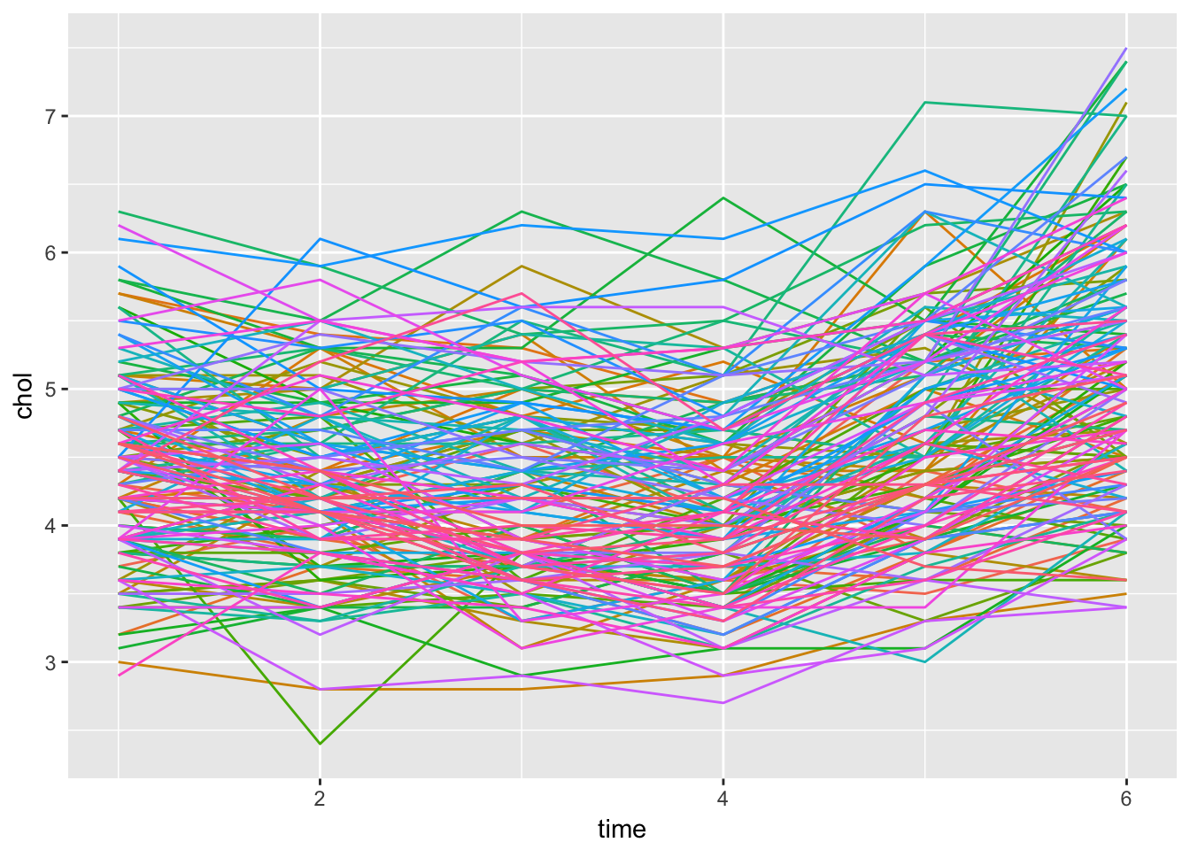

Twisk1 %>%
  ggplot(aes(x = time, y = chol, col = id)) + 
  geom_line() + 
  facet_grid(~gender) + 
  theme(legend.position = "none")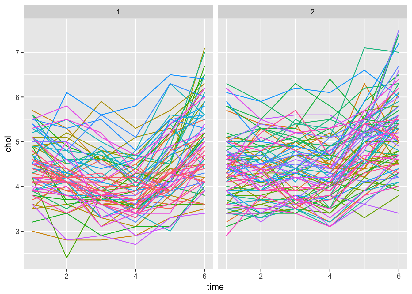

Using a split plot ANOVA, test whether cholesterol levels change in time. (From question d, does a linear time effect seem feasible?)

A linear time effect does not seem correct, based on the graph. We will use time as a factor variable

fit <- aov(chol~factor(time)+Error(id), data = Twisk1)
summary(fit)


Error: id
           Df Sum Sq Mean Sq F value Pr(>F)
Residuals 146  358.9   2.458               

Error: Within
              Df Sum Sq Mean Sq F value Pr(>F)    
factor(time)   5  91.06  18.211   100.6 <2e-16 ***
Residuals    730 132.11   0.181                   
---
Signif. codes:  0 '***' 0.001 '**' 0.01 '*' 0.05 '.' 0.1 ' ' 1

Is the effect of time for females the same as for males? Investigate by making an interaction plot and using split plot ANOVA.

We can already observe the ‘interaction’ from the faceted plot from ggplot. The slope seems equal for both sexes, which indicates no interaction

fit2 <- aov(chol~factor(time)*factor(gender)+Error(id), data = Twisk1)
summary(fit2)


Error: id
                Df Sum Sq Mean Sq F value Pr(>F)  
factor(gender)   1   15.2  15.159   6.394 0.0125 *
Residuals      145  343.8   2.371                 
---
Signif. codes:  0 '***' 0.001 '**' 0.01 '*' 0.05 '.' 0.1 ' ' 1

Error: Within
                             Df Sum Sq Mean Sq F value   Pr(>F)    
factor(time)                  5  91.06  18.211  105.46  < 2e-16 ***
factor(time):factor(gender)   5   6.92   1.385    8.02 2.26e-07 ***
Residuals                   725 125.19   0.173                     
---
Signif. codes:  0 '***' 0.001 '**' 0.01 '*' 0.05 '.' 0.1 ' ' 1

Here it seems that there is an important interaction with gender. Maybe if we plot the means on each time point, this will become apparant

Twisk1 %>% 
  group_by(time, gender) %>%
  summarize(chol = mean(chol)) %>%
  ggplot(aes(x = time, y = chol, col = gender)) + 
  geom_line()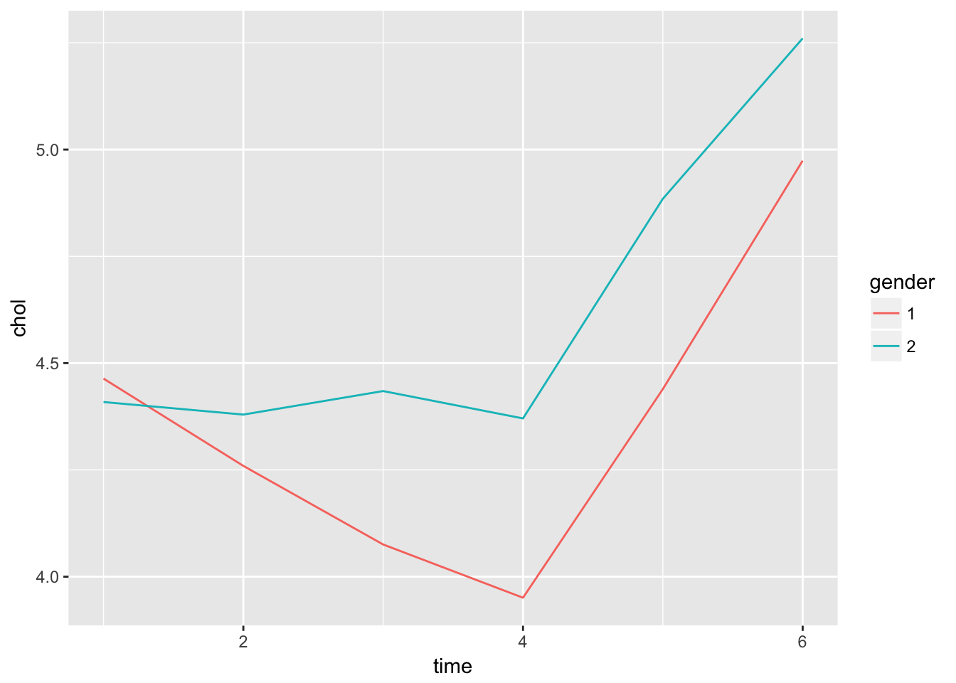

Redo questions e and f using a linear mixed effect model with a random intercept. Compare the outputs and conclusions to those from e and f).

First without interaction

fit.lme <- lme(fixed = chol~factor(time), random = ~1|id, data = Twisk1)
summary(fit.lme)

Linear mixed-effects model fit by REML
 Data: Twisk1 
       AIC      BIC    logLik
  1415.401 1453.604 -699.7004

Random effects:
 Formula: ~1 | id
        (Intercept) Residual
StdDev:   0.6160774 0.425416

Fixed effects: chol ~ factor(time) 
                  Value  Std.Error  DF  t-value p-value
(Intercept)    4.434694 0.06175055 730 71.81626  0.0000
factor(time)2 -0.111565 0.04962154 730 -2.24831  0.0249
factor(time)3 -0.168707 0.04962154 730 -3.39988  0.0007
factor(time)4 -0.261224 0.04962154 730 -5.26434  0.0000
factor(time)5  0.240816 0.04962154 730  4.85306  0.0000
factor(time)6  0.691156 0.04962154 730 13.92856  0.0000
 Correlation: 
              (Intr) fct()2 fct()3 fct()4 fct()5
factor(time)2 -0.402                            
factor(time)3 -0.402  0.500                     
factor(time)4 -0.402  0.500  0.500              
factor(time)5 -0.402  0.500  0.500  0.500       
factor(time)6 -0.402  0.500  0.500  0.500  0.500

Standardized Within-Group Residuals:
        Min          Q1         Med          Q3         Max 
-2.75247731 -0.58922213 -0.04251889  0.56513990  3.62717923 

Number of Observations: 882
Number of Groups: 147

Now with interaction

fit.lme2 <- lme(fixed = chol~factor(time)*gender, random = ~1|id, data = Twisk1)
summary(fit.lme2)

Linear mixed-effects model fit by REML
 Data: Twisk1 
       AIC      BIC    logLik
  1400.317 1467.076 -686.1587

Random effects:
 Formula: ~1 | id
        (Intercept)  Residual
StdDev:   0.6052576 0.4155439

Fixed effects: chol ~ factor(time) * gender 
                          Value  Std.Error  DF  t-value p-value
(Intercept)            4.463768 0.08838433 725 50.50407  0.0000
factor(time)2         -0.204348 0.07074689 725 -2.88844  0.0040
factor(time)3         -0.388406 0.07074689 725 -5.49008  0.0000
factor(time)4         -0.513043 0.07074689 725 -7.25182  0.0000
factor(time)5         -0.024638 0.07074689 725 -0.34825  0.7278
factor(time)6          0.510145 0.07074689 725  7.21085  0.0000
gender2               -0.054794 0.12133515 145 -0.45159  0.6522
factor(time)2:gender2  0.174861 0.09712224 725  1.80042  0.0722
factor(time)3:gender2  0.414047 0.09712224 725  4.26315  0.0000
factor(time)4:gender2  0.474582 0.09712224 725  4.88644  0.0000
factor(time)5:gender2  0.500279 0.09712224 725  5.15102  0.0000
factor(time)6:gender2  0.341137 0.09712224 725  3.51245  0.0005
 Correlation: 
                      (Intr) fct()2 fct()3 fct()4 fct()5 fct()6 gendr2
factor(time)2         -0.400                                          
factor(time)3         -0.400  0.500                                   
factor(time)4         -0.400  0.500  0.500                            
factor(time)5         -0.400  0.500  0.500  0.500                     
factor(time)6         -0.400  0.500  0.500  0.500  0.500              
gender2               -0.728  0.292  0.292  0.292  0.292  0.292       
factor(time)2:gender2  0.292 -0.728 -0.364 -0.364 -0.364 -0.364 -0.400
factor(time)3:gender2  0.292 -0.364 -0.728 -0.364 -0.364 -0.364 -0.400
factor(time)4:gender2  0.292 -0.364 -0.364 -0.728 -0.364 -0.364 -0.400
factor(time)5:gender2  0.292 -0.364 -0.364 -0.364 -0.728 -0.364 -0.400
factor(time)6:gender2  0.292 -0.364 -0.364 -0.364 -0.364 -0.728 -0.400
                      f()2:2 f()3:2 f()4:2 f()5:2
factor(time)2                                    
factor(time)3                                    
factor(time)4                                    
factor(time)5                                    
factor(time)6                                    
gender2                                          
factor(time)2:gender2                            
factor(time)3:gender2  0.500                     
factor(time)4:gender2  0.500  0.500              
factor(time)5:gender2  0.500  0.500  0.500       
factor(time)6:gender2  0.500  0.500  0.500  0.500

Standardized Within-Group Residuals:
        Min          Q1         Med          Q3         Max 
-3.16206297 -0.59878274 -0.01013853  0.53084464  3.76792278 

Number of Observations: 882
Number of Groups: 147

Again, we have an indication of significant interaction between time and gender.

After day 2: Formally compare the two LME model from part g, using AIC or a Likelihood Ratio test. (Note: we need to use ML instead of REML to get a valid comparison.) Also investigate a model with time and gender as main effects, without interaction. What happens if we leave out weeks 1 and 2?

First re-fit the model with package lme4, which supports the ANOVA method by re-fitting accordinging to REML

fit1 <- lme4::lmer(chol~factor(time) + (1|id), data = Twisk1)
fit2 <- lme4::lmer(chol~factor(time)*gender + (1|id), data = Twisk1)
fit3 <- lme4::lmer(chol~factor(time)+gender + (1|id), data = Twisk1)
fit4 <- lme4::lmer(chol~factor(time)+gender + (1|id), data = Twisk1 %>% filter(time > 2))

Compare with ANOVA (observe the message of refitting with ML)

Fit 2 is best, including interaction

anova(fit1, fit2, fit3)

Data: Twisk1
Models:
fit1: chol ~ factor(time) + (1 | id)
fit3: chol ~ factor(time) + gender + (1 | id)
fit2: chol ~ factor(time) * gender + (1 | id)
     Df    AIC    BIC  logLik deviance   Chisq Chi Df Pr(>Chisq)    
fit1  8 1388.8 1427.1 -686.41   1372.8                              
fit3  9 1384.5 1427.5 -683.24   1366.5  6.3436      1    0.01178 *  
fit2 14 1354.9 1421.9 -663.45   1326.9 39.5664      5  1.826e-07 ***
---
Signif. codes:  0 '***' 0.001 '**' 0.01 '*' 0.05 '.' 0.1 ' ' 1

Dependent data 2

1. Milk

In the protein example in the handout there where 4 timepoints. In the actual dataset there were much points. To select 7 timepoints from the data:

library(nlme)
milk<-Milk[Milk$Time<8,]
str(milk)

Classes 'nfnGroupedData', 'nfGroupedData', 'groupedData' and 'data.frame':  549 obs. of  4 variables:
 $ protein: num  3.63 3.57 3.47 3.65 3.89 3.73 3.77 3.24 3.25 3.29 ...
 $ Time   : num  1 2 3 4 5 6 7 1 2 3 ...
 $ Cow    : Ord.factor w/ 79 levels "B04"<"B14"<"B03"<..: 25 25 25 25 25 25 25 4 4 4 ...
 $ Diet   : Factor w/ 3 levels "barley","barley+lupins",..: 1 1 1 1 1 1 1 1 1 1 ...
 - attr(*, "formula")=Class 'formula'  language protein ~ Time | Cow
  .. ..- attr(*, ".Environment")=<environment: R_GlobalEnv> 
 - attr(*, "labels")=List of 2
  ..$ x: chr "Time since calving"
  ..$ y: chr "Protein content of milk sample"
 - attr(*, "units")=List of 2
  ..$ x: chr "(weeks)"
  ..$ y: chr "(%)"
 - attr(*, "outer")=Class 'formula'  language ~Diet
  .. ..- attr(*, ".Environment")=<environment: R_GlobalEnv> 
 - attr(*, "FUN")=function (x)  
 - attr(*, "order.groups")= logi TRUE

1.  Fit the model with Diet and time as grouping variables, and
    their interaction. For the random part take random intercepts
    and random slopes.

require(lme4)
fit1 <- lmer(protein~Diet*factor(Time) + (Time | Cow), data = milk)
summary(fit1)

Linear mixed model fit by REML ['lmerMod']
Formula: protein ~ Diet * factor(Time) + (Time | Cow)
   Data: milk

REML criterion at convergence: 99.8

Scaled residuals: 
    Min      1Q  Median      3Q     Max 
-3.3577 -0.5317  0.0259  0.5411  3.1318 

Random effects:
 Groups   Name        Variance Std.Dev. Corr 
 Cow      (Intercept) 0.081159 0.28488       
          Time        0.001993 0.04465  -0.71
 Residual             0.040877 0.20218       
Number of obs: 549, groups:  Cow, 79

Fixed effects:
                                 Estimate Std. Error t value
(Intercept)                      3.886800   0.065076   59.73
Dietbarley+lupins               -0.025689   0.090310   -0.28
Dietlupins                      -0.128652   0.090310   -1.42
factor(Time)2                   -0.249561   0.058621   -4.26
factor(Time)3                   -0.388800   0.059909   -6.49
factor(Time)4                   -0.510400   0.063149   -8.08
factor(Time)5                   -0.402400   0.067423   -5.97
factor(Time)6                   -0.500400   0.072550   -6.90
factor(Time)7                   -0.418000   0.078361   -5.33
Dietbarley+lupins:factor(Time)2 -0.071550   0.080859   -0.88
Dietlupins:factor(Time)2        -0.080809   0.080859   -1.00
Dietbarley+lupins:factor(Time)3 -0.126756   0.083140   -1.52
Dietlupins:factor(Time)3         0.003615   0.083140    0.04
Dietbarley+lupins:factor(Time)4 -0.072933   0.087636   -0.83
Dietlupins:factor(Time)4         0.046326   0.087636    0.53
Dietbarley+lupins:factor(Time)5 -0.120933   0.093568   -1.29
Dietlupins:factor(Time)5        -0.111324   0.093930   -1.19
Dietbarley+lupins:factor(Time)6  0.031881   0.100683    0.32
Dietlupins:factor(Time)6         0.022622   0.100683    0.22
Dietbarley+lupins:factor(Time)7 -0.109778   0.108748   -1.01
Dietlupins:factor(Time)7        -0.130901   0.109542   -1.19

2.  See, by fitting different models, which random effects are
    needed in the model. (Just like in the text.)

fit2 <- lmer(protein~Diet*factor(Time) + (Time - 1 | Cow), data = milk)
fit3 <- lmer(protein~Diet*factor(Time) + (1 | Cow), data = milk)

anova(fit1, fit2, fit3)

Data: milk
Models:
fit2: protein ~ Diet * factor(Time) + (Time - 1 | Cow)
fit3: protein ~ Diet * factor(Time) + (1 | Cow)
fit1: protein ~ Diet * factor(Time) + (Time | Cow)
     Df     AIC    BIC  logLik deviance  Chisq Chi Df Pr(>Chisq)    
fit2 23 154.214 253.30 -54.107  108.214                             
fit3 23  84.518 183.60 -19.259   38.518 69.697      0  < 2.2e-16 ***
fit1 25  61.123 168.82  -5.561   11.123 27.395      2  1.125e-06 ***
---
Signif. codes:  0 '***' 0.001 '**' 0.01 '*' 0.05 '.' 0.1 ' ' 1

Fit1 is best, so both random slope and intercept are needed

3.  See, by fitting different models, what the fixed part of the
    model is.

fit4 <- lmer(protein~Diet+factor(Time) + (Time | Cow), data = milk)
fit5 <- lmer(protein~Diet+Diet:factor(Time) + (Time | Cow), data = milk)
fit6 <- lmer(protein~Diet + (Time | Cow), data = milk)
fit7 <- lmer(protein~factor(Time) + (Time | Cow), data = milk)

anova(fit1, fit4, fit5, fit6, fit7)

Data: milk
Models:
fit6: protein ~ Diet + (Time | Cow)
fit7: protein ~ factor(Time) + (Time | Cow)
fit4: protein ~ Diet + factor(Time) + (Time | Cow)
fit1: protein ~ Diet * factor(Time) + (Time | Cow)
fit5: protein ~ Diet + Diet:factor(Time) + (Time | Cow)
     Df     AIC    BIC   logLik deviance    Chisq Chi Df Pr(>Chisq)    
fit6  7 235.792 265.95 -110.896  221.792                               
fit7 11  57.020 104.41  -17.510   35.020 186.7726      4    < 2e-16 ***
fit4 13  53.310 109.31  -13.655   27.310   7.7096      2    0.02118 *  
fit1 25  61.123 168.82   -5.561   11.123  16.1876     12    0.18279    
fit5 25  61.123 168.82   -5.561   11.123   0.0000      0    1.00000    
---
Signif. codes:  0 '***' 0.001 '**' 0.01 '*' 0.05 '.' 0.1 ' ' 1

Fit4 has the lowest AIC, without interaction between time and diet

4.  Discuss the difference with the analysis from the text and
    explain this.

length(unique(Milk$Time))

[1] 19

length(unique(milk$Time))

[1] 7

In the full dataset there are 19 unique datapoints, in the dataset we used, this was restricted to 7. This could explain why the interaction is not significant when there are only few timepoint (maybe the interesting interaction is at later time-points)

Try a plot

Milk %>%
  group_by(Time, Diet) %>%
  summarize(protein = mean(protein)) %>%
  ggplot(aes(x = Time, y = protein, col = Diet)) + 
  geom_line() +
  theme(legend.position = "none")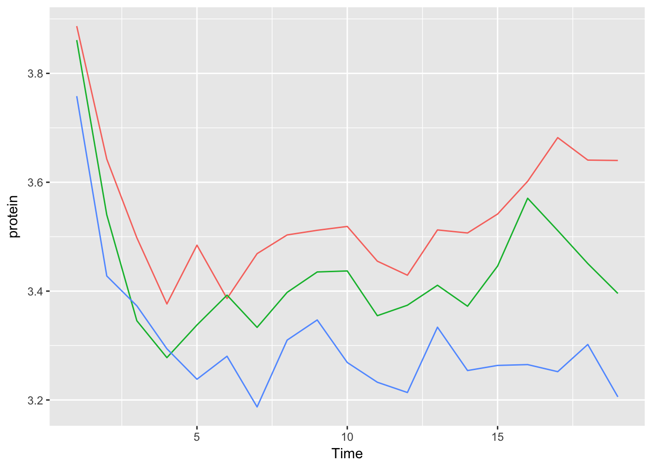

We can more or less see that the slopes start to differ after timepoint 7.

Notice that individual cows were left out here

2.

In the nlme library there is a dataset on the body weights of rats, measured over 64 days. The body weights of the rats (in grams) are measured on day 1 and every seven days thereafter until day64, with an extra measurement on day 44. The experiment started several weeks before “day 1.” There are three groups of rats, each on a different diet. The dataset is named BodyWeight. In this dataset Diet is a factor, the other variables are numeric covariates.

1.  Attach the BodyWeight dataset, get information about this
    dataset (help(BodyWeight)) and make a plot like figure 1 of the
    handout.

data("BodyWeight")
str(BodyWeight)

Classes 'nfnGroupedData', 'nfGroupedData', 'groupedData' and 'data.frame':  176 obs. of  4 variables:
 $ weight: num  240 250 255 260 262 258 266 266 265 272 ...
 $ Time  : num  1 8 15 22 29 36 43 44 50 57 ...
 $ Rat   : Ord.factor w/ 16 levels "2"<"3"<"4"<"1"<..: 4 4 4 4 4 4 4 4 4 4 ...
 $ Diet  : Factor w/ 3 levels "1","2","3": 1 1 1 1 1 1 1 1 1 1 ...
 - attr(*, "outer")=Class 'formula'  language ~Diet
  .. ..- attr(*, ".Environment")=<environment: R_GlobalEnv> 
 - attr(*, "formula")=Class 'formula'  language weight ~ Time | Rat
  .. ..- attr(*, ".Environment")=<environment: R_GlobalEnv> 
 - attr(*, "labels")=List of 2
  ..$ x: chr "Time"
  ..$ y: chr "Body weight"
 - attr(*, "units")=List of 2
  ..$ x: chr "(days)"
  ..$ y: chr "(g)"
 - attr(*, "FUN")=function (x)  
  ..- attr(*, "source")= chr "function(x) max(x, na.rm = TRUE)"
 - attr(*, "order.groups")= logi TRUE

Spaghetti plot:

BodyWeight %>%
  ggplot(aes(x = Time, y = weight, col = Rat)) + 
  geom_line() + 
  facet_wrap(~Diet) + 
  theme(legend.position = "none")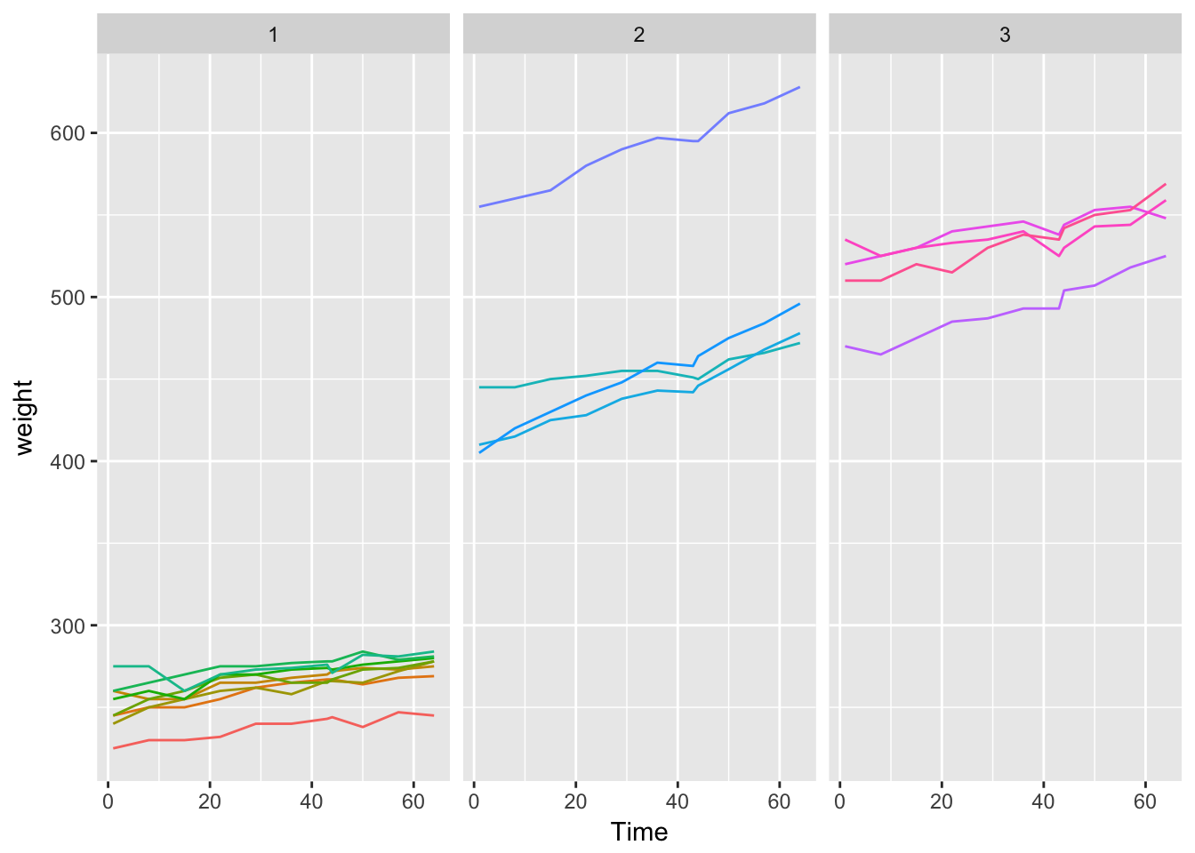

2.  Which random effects are needed in the model? Take for the fixed
    part a model with Diet and Time as grouping variables, and their
    interaction.

Intercepts seem to differ by rat, slopes not too much. Intercepts are all pretty different for diets (remember that the rats were already on a diet for sometime before Time = 0)

library(lme4)
fit1 <- lmer(weight~Diet*factor(Time) + (1|Rat), data = BodyWeight)
fit2 <- lmer(weight~Diet*factor(Time) + (Time - 1|Rat), data = BodyWeight)
fit3 <- lmer(weight~Diet*factor(Time) + (Time|Rat), data = BodyWeight)

AIC(fit1, fit2, fit3)

     df      AIC
fit1 35 1132.813
fit2 35 1426.671
fit3 37 1035.145

Fit3 is best, including random intercept and slope

3.  Check which fixed parts are needed in the model.

fit4 <- lmer(weight~Diet+factor(Time) + (Time|Rat), data = BodyWeight)
fit5 <- lmer(weight~Diet+Diet:factor(Time) + (Time|Rat), data = BodyWeight)
fit6 <- lmer(weight~Diet + (Time|Rat), data = BodyWeight)
fit7 <- lmer(weight~factor(Time) + (Time|Rat), data = BodyWeight)

anova(fit3, fit4, fit5, fit6, fit7)

Data: BodyWeight
Models:
fit6: weight ~ Diet + (Time | Rat)
fit7: weight ~ factor(Time) + (Time | Rat)
fit4: weight ~ Diet + factor(Time) + (Time | Rat)
fit3: weight ~ Diet * factor(Time) + (Time | Rat)
fit5: weight ~ Diet + Diet:factor(Time) + (Time | Rat)
     Df    AIC    BIC  logLik deviance  Chisq Chi Df Pr(>Chisq)    
fit6  7 1214.1 1236.3 -600.07   1200.1                             
fit7 15 1212.5 1260.1 -591.26   1182.5 17.610      8    0.02434 *  
fit4 17 1181.0 1234.9 -573.52   1147.0 35.483      2  1.972e-08 ***
fit3 37 1154.7 1272.0 -540.36   1080.7 66.326     20  7.163e-07 ***
fit5 37 1154.7 1272.0 -540.36   1080.7  0.000      0    1.00000    
---
Signif. codes:  0 '***' 0.001 '**' 0.01 '*' 0.05 '.' 0.1 ' ' 1

Fit 4 is best, with fixed effects for time and diet but no interaction

4.  Determine the correlation between the observations on the
    different time points and discuss these.

Go back to package nlme for this

fit <- nlme::lme(fixed = weight~Diet+factor(Time),
                  random = (~Time|Rat), 
                  data = BodyWeight)

covmat <- nlme::getVarCov(fit, individual = 1, type = "marginal")
covmat

Rat 1 
Marginal variance covariance matrix
        1      2      3      4      5      6      7      8      9     10
1  1407.9 1372.7 1354.4 1336.1 1317.9 1299.6 1281.4 1278.8 1263.1 1244.9
2  1372.7 1377.3 1348.0 1335.6 1323.3 1310.9 1298.6 1296.8 1286.2 1273.9
3  1354.4 1348.0 1358.5 1335.1 1328.7 1322.2 1315.8 1314.9 1309.4 1302.9
4  1336.1 1335.6 1335.1 1351.5 1334.0 1333.5 1333.0 1332.9 1332.5 1331.9
5  1317.9 1323.3 1328.7 1334.0 1356.4 1344.8 1350.2 1351.0 1355.6 1361.0
6  1299.6 1310.9 1322.2 1333.5 1344.8 1373.1 1367.4 1369.0 1378.7 1390.0
7  1281.4 1298.6 1315.8 1333.0 1350.2 1367.4 1401.6 1387.1 1401.8 1419.0
8  1278.8 1296.8 1314.9 1332.9 1351.0 1369.0 1387.1 1406.6 1405.1 1423.2
9  1263.1 1286.2 1309.4 1332.5 1355.6 1378.7 1401.8 1405.1 1441.9 1448.1
10 1244.9 1273.9 1302.9 1331.9 1361.0 1390.0 1419.0 1423.2 1448.1 1494.0
11 1226.6 1261.5 1296.5 1331.4 1366.4 1401.3 1436.2 1441.2 1471.2 1506.1
       11
1  1226.6
2  1261.5
3  1296.5
4  1331.4
5  1366.4
6  1401.3
7  1436.2
8  1441.2
9  1471.2
10 1506.1
11 1558.0
  Standard Deviations: 37.522 37.112 36.858 36.763 36.829 37.055 37.438 37.505 37.972 38.653 39.472

We can see that covariance decreases with increasing time difference. We can plot this nicely:

image(covmat[[1]])

In the edges of the matrix, the color is more yellow, which indicates lower covariance

5.  Describe the analysis you did, and the conclusions that can be
    drawn.

Left to reader

3. Osteochon

Read in the data file osteochon.csv.

ost <- read.csv(fromParentDir("data/osteochon.csv"))
str(ost)

'data.frame':   440 obs. of  5 variables:
 $ father: int  1 1 1 1 1 1 1 1 1 1 ...
 $ food  : int  3 2 1 2 2 1 1 2 2 2 ...
 $ ground: int  2 1 2 1 1 2 2 1 1 2 ...
 $ height: int  166 165 160 163 161 155 162 166 162 164 ...
 $ oc    : int  0 0 1 0 0 0 0 0 0 0 ...

Make father and food factors

ost %<>%
  mutate(father = factor(father), ground = factor(ground))

1.  Fit a logistic regression model with independent variables
    father, ground and height. (Remember to use factor() for father
    and ground.)

fit <- glm(oc~father+ground+height, data = ost,
           family = binomial)

2.  Discuss the estimates and standard errors for the fathers.

summary(fit)


Call:
glm(formula = oc ~ father + ground + height, family = binomial, 
    data = ost)

Deviance Residuals: 
     Min        1Q    Median        3Q       Max  
-1.30706  -0.60192  -0.42928  -0.00014   2.64714  

Coefficients:
              Estimate Std. Error z value Pr(>|z|)   
(Intercept)  -21.05269    6.45772  -3.260  0.00111 **
father2       -0.39502    1.07838  -0.366  0.71413   
father3        0.27001    1.08908   0.248  0.80420   
father4        1.24442    0.98298   1.266  0.20553   
father5      -16.29436 1928.64557  -0.008  0.99326   
father6       -0.47822    1.07903  -0.443  0.65763   
father7        0.88621    0.94082   0.942  0.34622   
father8        0.14027    1.08704   0.129  0.89732   
father9       -0.36745    1.07149  -0.343  0.73165   
father10       0.26745    1.00977   0.265  0.79111   
father11       0.05222    1.09061   0.048  0.96181   
father12     -17.04994 1641.37585  -0.010  0.99171   
father13       0.96627    1.03021   0.938  0.34828   
father14     -17.07564 1861.39065  -0.009  0.99268   
father15     -16.69329 1607.14164  -0.010  0.99171   
father16      -0.82301    1.28847  -0.639  0.52299   
father17     -16.50985 1770.66337  -0.009  0.99256   
father18       0.31936    1.01990   0.313  0.75418   
father19       0.51245    1.02260   0.501  0.61628   
father20       0.91762    1.02921   0.892  0.37262   
father21      -0.98278    1.29515  -0.759  0.44796   
father22      -0.29347    1.08335  -0.271  0.78648   
father23      -1.47928    1.31366  -1.126  0.26013   
father24       0.18565    0.99817   0.186  0.85245   
father25       0.72438    0.95492   0.759  0.44810   
father26       0.11776    1.07700   0.109  0.91293   
father27       0.99152    1.00069   0.991  0.32176   
father28      -0.26350    1.08649  -0.243  0.80838   
father29       0.84449    0.99059   0.853  0.39393   
father30     -16.71132 1952.56764  -0.009  0.99317   
ground2        0.36450    0.32161   1.133  0.25706   
height         0.11586    0.03913   2.961  0.00306 **
---
Signif. codes:  0 '***' 0.001 '**' 0.01 '*' 0.05 '.' 0.1 ' ' 1

(Dispersion parameter for binomial family taken to be 1)

    Null deviance: 361.41  on 439  degrees of freedom
Residual deviance: 305.36  on 408  degrees of freedom
AIC: 369.36

Number of Fisher Scoring iterations: 17

There are many fathers, none are significant. Some have high values, but also very high standard errors.

3.  Now fit a logistic regression model with random father effects.

This model wouldn’t converge and suggested scaling, so height was centered (to mean 0, variance unchanged)

ost %<>% 
  mutate(height_centered = scale(height, center = T, scale = F))

fit2 <- lme4::glmer(oc ~ height_centered+food + (1|father), 
                    data = ost,
                    family = binomial)

fit3 <- lme4::glmer(oc ~ height_centered+food + 
                      (height_centered|father), 
                    data = ost,
                    family = binomial)

summary(fit2)

Generalized linear mixed model fit by maximum likelihood (Laplace
  Approximation) [glmerMod]
 Family: binomial  ( logit )
Formula: oc ~ height_centered + food + (1 | father)
   Data: ost

     AIC      BIC   logLik deviance df.resid 
   360.1    376.5   -176.1    352.1      436 

Scaled residuals: 
    Min      1Q  Median      3Q     Max 
-0.8435 -0.4278 -0.3674 -0.2926  4.4019 

Random effects:
 Groups Name        Variance Std.Dev.
 father (Intercept) 0.1595   0.3994  
Number of obs: 440, groups:  father, 30

Fixed effects:
                Estimate Std. Error z value Pr(>|z|)    
(Intercept)     -1.76975    0.52791  -3.352 0.000801 ***
height_centered  0.09944    0.03480   2.857 0.004271 ** 
food            -0.05959    0.23824  -0.250 0.802490    
---
Signif. codes:  0 '***' 0.001 '**' 0.01 '*' 0.05 '.' 0.1 ' ' 1

Correlation of Fixed Effects:
            (Intr) hght_c
heght_cntrd  0.045       
food        -0.944 -0.139

4.  Compare the AIC’s of both models and discuss which model fits
    best. Also compare the estimates of height.

AIC(fit, fit2, fit3)

     df      AIC
fit  32 369.3610
fit2  4 360.1499
fit3  6 363.7779

AIC is the lowest for fit2. The estimates of beta for height are pretty similar in both models, but even stronger in fit2

5.  Discuss the effect of using random father effects.

list(fit, fit2) %>%
  map(logLik)

[[1]]
'log Lik.' -152.6805 (df=32)

[[2]]
'log Lik.' -176.075 (df=4)

When looking at the likelihood of the models, fit has a better likelihood, however, it ‘spends’ many degrees of freedom on estimating fixed effects for each father. The model with random effects (fit2) has a lot less parameters to estimate, which gives it a better AIC and makes it preferable to the model without random effects.

Session information

sessionInfo()

R version 3.4.3 (2017-11-30)
Platform: x86_64-apple-darwin15.6.0 (64-bit)
Running under: macOS Sierra 10.12.6

Matrix products: default
BLAS: /Library/Frameworks/R.framework/Versions/3.4/Resources/lib/libRblas.0.dylib
LAPACK: /Library/Frameworks/R.framework/Versions/3.4/Resources/lib/libRlapack.dylib

locale:
[1] en_US.UTF-8/en_US.UTF-8/en_US.UTF-8/C/en_US.UTF-8/en_US.UTF-8

attached base packages:
[1] stats     graphics  grDevices utils     datasets  methods   base     

other attached packages:
 [1] lme4_1.1-15         Matrix_1.2-12       lattice_0.20-35    
 [4] nlme_3.1-131        data.table_1.10.4-3 survival_2.41-3    
 [7] bindrcpp_0.2        simpleboot_1.1-3    boot_1.3-20        
[10] purrr_0.2.4         stringr_1.2.0       ggplot2_2.2.1      
[13] dplyr_0.7.4         magrittr_1.5        epistats_0.1.0     

loaded via a namespace (and not attached):
 [1] reshape2_1.4.3   splines_3.4.3    colorspace_1.3-2 htmltools_0.3.6 
 [5] yaml_2.1.16      utf8_1.1.3       rlang_0.1.6      nloptr_1.0.4    
 [9] pillar_1.1.0     foreign_0.8-69   glue_1.2.0       bindr_0.1       
[13] plyr_1.8.4       munsell_0.4.3    gtable_0.2.0     codetools_0.2-15
[17] psych_1.7.8      evaluate_0.10.1  labeling_0.3     knitr_1.19      
[21] parallel_3.4.3   broom_0.4.3      Rcpp_0.12.15     scales_0.5.0    
[25] backports_1.1.2  mnormt_1.5-5     digest_0.6.15    stringi_1.1.6   
[29] grid_3.4.3       rprojroot_1.3-2  cli_1.0.0        tools_3.4.3     
[33] perm_1.0-0.0     lazyeval_0.2.1   tibble_1.4.2     crayon_1.3.4    
[37] tidyr_0.8.0      pkgconfig_2.0.1  MASS_7.3-48      assertthat_0.2.0
[41] minqa_1.2.4      rmarkdown_1.8    R6_2.2.2         git2r_0.21.0    
[45] compiler_3.4.3

This R Markdown site was created with workflowr