library(mice)
library(ggplot2); theme_set(theme_bw())

df <- boys

nimps <- 5
imp <- mice(df, m = nimps, method = "pmm")In an earlier blog post I show how to plot the dependence of a response variable on covariate, both conditional on other covariates with a partial residual plot In this post I investigate how to do this when there are missing values using package mice.
This post will rely in Hanne Oberman’s vignette on ggmice, a plotting package for mice::mids objects.
Data and imputation
In this post we’ll use the boys dataset which is provided in the mice package. The mice package implements multiple imputation through chained equations1.
Partial residual plot with complete data
We’ll assume we’re interested in how weight (wgt) depends on height (hgt), corrected for all other variables. Both have missing values in the dataset.
We can use one of the imputed datasets to show how partial residual plots are made with complete data. With complete data, partial residual plots can be created like so:
df1 <- complete(imp, 1)

get_partial_resid <- function(data) {
  fit <- lm(wgt~., data=data)
  yresid <- resid(fit)
  return(yresid + coef(fit)['hgt'] * data$hgt)
}

plotdata1 <- data.frame(hgt=df1$hgt, y=get_partial_resid(df1))

ggplot(plotdata1, aes(x=hgt, y=y)) + geom_point()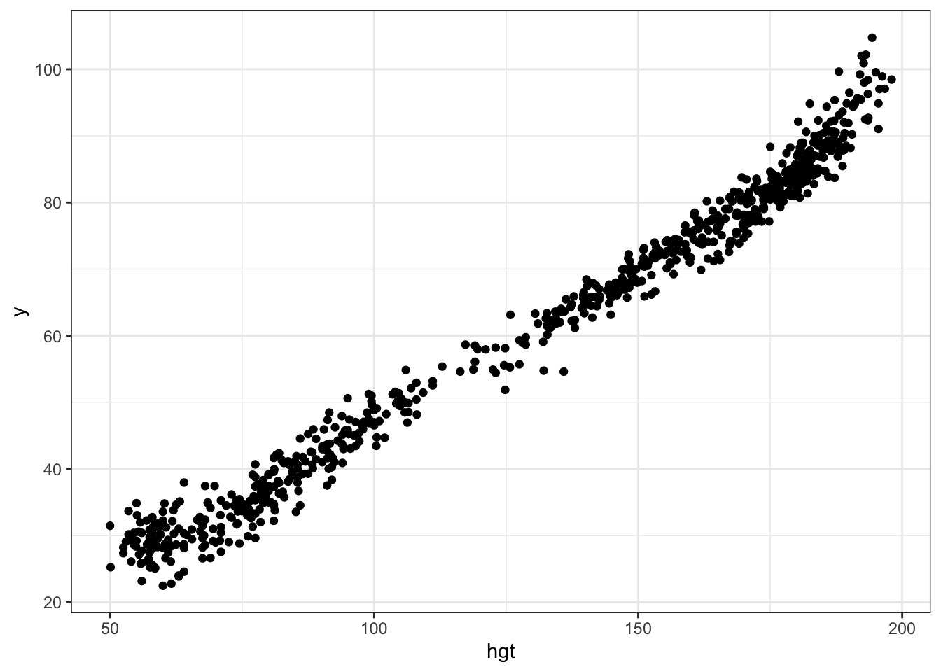
Note how this differs from the marginal association between hgt and wgt. The difference between the plots is explained by other covariates that are correlated both with hgt and wgt.
ggplot(df1, aes(x=hgt, y=wgt)) + geom_point()
Putting them together
The issue with the partial residual plot Figure 1 is that the residuals depend on the imputed values for all variables. How to go about this? We can treat the residuals as we would ‘coefficients’ in imputation and use Rubin’s rules on them. Let’s see how to do this with mice.
impdfs <- complete(imp, "all")
impdfs <- lapply(impdfs, function(data) data.frame(data, partial_resid=get_partial_resid(data)))
impdfs <- lapply(1:nimps, function(i) data.frame(impdfs[[i]], impidx=i))
impdf_long <- do.call(rbind, impdfs)
Note that we cannot directly pool the residuals because they may be correlated with the imputed values for hgt. Pooling imputed values for hgt and the partial residual removes this correlation. Instead we could just plot all the values.
ggplot(impdf_long, aes(x=hgt, y=partial_resid)) + geom_point(aes(shape=factor(impidx)), alpha=0.5)
In the future I’d like to learn how to make good bivariate estimates of these points (e.g. fitting a bivariate normal distribution). This should for example also come up in calculating sensitivity and specificity on multiply imputed datasets, as these are clearly correlated. Fully bayesian imputation is another possibility obviously.
Footnotes
multiple imputation with chained equations sequentially imputes values for all variables with missing values by building prediction models for each variable based on other variables. This imputation is done multiple times with multiple random seeds and thus results in a number of different imputed datasets. A typical analysis workflow is to do these imputations and on each imputed dataset fit a model of interest. The coefficients of these models can then be pooled using Rubin’s rules.↩︎
Citation
BibTeX citation:
@online{van amsterdam,
  author = {van Amsterdam, Wouter},
  title = {Partial Residual Plots with Multiply Imputed Data},
  url = {https://vanamsterdam.github.io/posts/240322-mice-partial-residual-plot.html},
  langid = {en}
}
For attribution, please cite this work as:
Amsterdam, Wouter van. n.d. “Partial Residual Plots with Multiply
Imputed Data.” https://vanamsterdam.github.io/posts/240322-mice-partial-residual-plot.html.